BC3203
Week 9 Coding Lecture
Interpreting Differential Expression results
library(tidyverse)
For this exercise you will need access to a small number of data files. Obtain these as follows;
wget "https://cloudstor.aarnet.edu.au/plus/s/eV9aZppq4f9AEdo/download" -O data.tgz
tar -zxvf data.tgz
Our starting point is a table of genes or proteins. We’ll work with a table of differentially expressed Mouse proteins from the RNASeq assignment.
mm_de <- read_tsv("data/rnaseq.tsv")
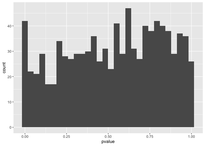
Note that this list includes all genes with enough data to measure expression reliably. In other words it includes both differentially expressed genes and those that are not differentially expressed.
We can see this by looking at a histogram of p-values which spans the entire range from 0 through to 1.
ggplot(mm_de,aes(x=pvalue)) + geom_histogram()
Our goal is to perform biological interpretation on these genes. In
order to do this we will need to use the gene identifiers (eg
ENSMUSG00000002455) to look up information about function. We will do
this using the Uniprot mapping service
First extract only the identifiers
cat data/rnaseq.tsv | awk '{print $1}' > data/ensids.txt
Next upload the ids to the Uniprot ID Mapping service at https://www.uniprot.org/uploadlists/

After converting IDs you should see that around 870 of our 943 are mapped. (Why not all of them?)
Note that the mapping is not 1:1 at all. Some Ensembl IDs have no equivalent in Uniprot (eg if they are non-coding genes) and some Ensembl IDs will have map to multiple uniprot entries. Many of the multi-mappings occur because unreviewed transcripts are included in the initial search results. Remove these by selecting only Reviewed proteins (Swiss-Prot).
Now dowload the table of information about each of the proteins in
excel format and save it to the data/uniprot.xlsx.
We can read this table in using tidyverse.
mm_sp <- readxl::read_xlsx("data/uniprot.xlsx")
Let’s also do some clean up as follows;
- Fix column names to make them R compatible
- Select only the columns we will need for this exercise.
- Pick only the first entry for each distinct gene id. (This is less than ideal. What other strategies are there?)
mm_sp <- readxl::read_xlsx("data/uniprot.xlsx") %>%
  select(ens_id = 1, protein_names = `Protein names`, gene_names = `Gene names`, go_terms = `Gene ontology IDs`) %>%
  group_by(ens_id) %>%
  summarise(protein_names=first(protein_names), gene_names=first(gene_names), go_terms=first(go_terms))
Join this with our differential expression data
mm_de_sp <- mm_de %>%
  left_join(mm_sp,by = c("gene_id"="ens_id"))
There is not much we can do with unannotated entries so we just remove them. This will do for now but in a real project you would go to greater lengths to ensure that the maximum number of genes are annotated.
mm_de_sp <- mm_de %>%
  left_join(mm_sp,by = c("gene_id"="ens_id")) %>%
  filter(!is.na(go_terms))
GO term enrichment analysis
As mentioned in lectures there are many different GO term analysis
packages with different strengths and weaknesses. Here I will focus on
the topGO package. It’s strength is that is uses a weighting method to
reduce the correlation structure induced by connections between terms in
the GO graph. From a practical point of view this means that it will
tend to focus on more specific GO terms (ie those further down in the GO
hierarchy) and these tend to be more useful for interpretation.
Note: Since this is RNASeq data it includes a bias towards inclusion
of longer genes in the target set. For a real analysis a package such as
goseq which accounts for this should be used.
Non-Tidyverse Code: The code below follows some patterns that I
would normally avoid such as updating a variable after creating it (best
avoided using pipes). In this case the requirements of the topGO
package don’t lend themselves to my preferred coding patterns. In the
interest of pragmatism I have adopted the topGO way of doing things
for some of the code below.
topGO requires a mapping between genes and go terms in the form of a
named list. Each item in the list should be a vector of go_terms for a
gene.
We can extract the important parts of this from our data as follows;
gene_ids <- mm_de_sp$gene_id
gostrings <- mm_de_sp$go_terms
Now convert the ; separated strings for each gene into a vector and
make these into a named list where the names are the gene ids
gostring2vector <- function(gostring){
   str_split(gostring,";")[[1]] %>% str_trim()
}


geneID2GO <- lapply(gostrings,gostring2vector)
names(geneID2GO) <- gene_ids
Next we extract only the significant genes. We want another named
vector. This time names are gene_ids but the values are TRUE or
FALSE indicating whether that gene is part of the target set.
significant_genes <- mm_de_sp %>%
  filter(padj<0.01) %>%
  pull(gene_id)

target_list_membership <- factor(as.integer(gene_ids %in% significant_genes))
names(target_list_membership) <- gene_ids
Now some highly specific steps which are idiosyncratic to the topGO
package. We first create a topGOdata object which captures all the
information about our enrichment.
Note the choice of Ontology here as BP. GO defines three separate
ontologies as explained in it’s
documentation
| Ontology Name | topGO abbreviation |
Meaning |
|---|---|---|
| Biological Process | BP | The larger processes, or ‘biological programs’ accomplished by multiple molecular activities |
| Molecular Function | MF | Molecular-level activities performed by gene products |
| Cellular Component | CC | The locations relative to cellular structures in which a gene product performs a function |
# Installing topGO
# Since topGO is a bioconductor package you can install it with this code
if (!requireNamespace("BiocManager", quietly = TRUE))
    install.packages("BiocManager")

BiocManager::install("topGO")
library(topGO)

GOdata <- new("topGOdata",
                  ontology = "BP",
                  allGenes = target_list_membership,
                  annot = annFUN.gene2GO,
                  gene2GO = geneID2GO,
                  nodeSize = 5)
Statistical testing is performed with Fisher’s exact test after applying
topGO weights to emphasise more specific terms.
# This runs the test to see if there are significantly enriched GO terms
resultFis <- runTest(GOdata, algorithm = "weight01", statistic = "fisher")

# This extracts test results to a table
gt <- GenTable(GOdata, classic = resultFis,orderBy = "weight", ranksOf = "classic", topNodes = 50)
Looking at gt there are a couple of significantly enriched GO terms.
The top one is GO:0032731
if (!requireNamespace("BiocManager", quietly = TRUE))
    install.packages("BiocManager")

BiocManager::install("Rgraphviz")
For the purposes of understanding the GO hierarchy it’s useful to view the graph of terms. Here we select the top 2 enriched terms and plot all connected nodes.
showSigOfNodes(GOdata, score(resultFis),firstSigNodes = 2)
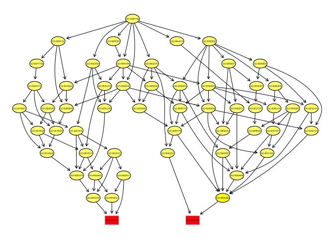
## $dag
## A graphNEL graph with directed edges
## Number of Nodes = 55
## Number of Edges = 117
##
## $complete.dag
## [1] "A graph with 55 nodes."
This graph is actually remarkably specific. Generally the terminal (highly specific) terms are enriched (red). This situation reflects the highly targeted nature of the experiment but other types of experiments might yield a more general enrichment pattern with enrichment at higher nodes.
What about the other ontologies. There are “MF” and “CC”
GOdataMF <- new("topGOdata",
                  ontology = "MF",
                  allGenes = target_list_membership,
                  annot = annFUN.gene2GO,
                  gene2GO = geneID2GO,
                  nodeSize = 5)

# This runs the test to see if there are significantly enriched GO terms
resultFisMF <- runTest(GOdataMF, algorithm = "weight01", statistic = "fisher")

# This extracts test results to a table .. the results actually look quite interesting .. :)
gtmf <- GenTable(GOdataMF, classic = resultFisMF,orderBy = "weight", ranksOf = "classic", topNodes = 50)
GOdataCC <- new("topGOdata",
                  ontology = "CC",
                  allGenes = target_list_membership,
                  annot = annFUN.gene2GO,
                  gene2GO = geneID2GO,
                  nodeSize = 5)

# This runs the test to see if there are significantly enriched GO terms
resultFisCC <- runTest(GOdataCC, algorithm = "weight01", statistic = "fisher")

# This extracts test results to a table .. the results actually look quite interesting .. :)
gtcc <- GenTable(GOdataCC, classic = resultFisCC,orderBy = "weight", ranksOf = "classic", topNodes = 50)
Exploring enrichment in more detail
Let’s tidy the data by splitting the GO term column
mm_de_sp_tidy <- mm_de_sp %>%
  separate_rows(go_terms, sep=";") %>%
  mutate(go_terms = str_trim(go_terms))
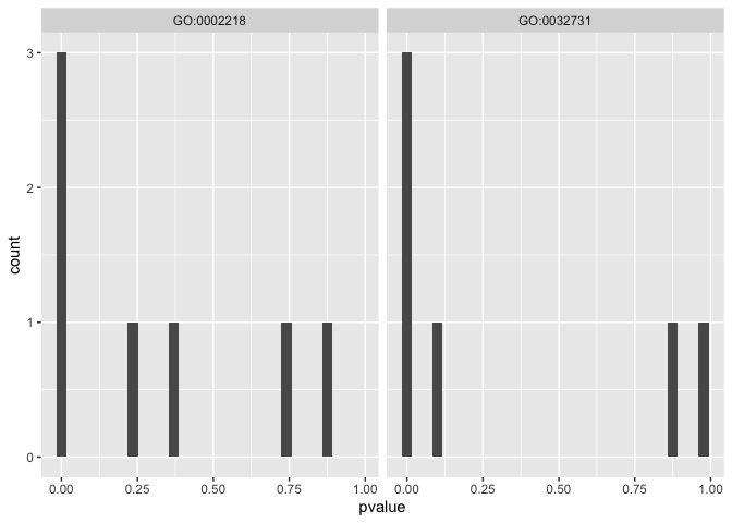
This now allows us to plot a histogram of p-values for differential expression of genes with any particular GO term.
significant_go_terms_gt <- gt %>%
  filter(classic<0.01) %>%
  pull(`GO.ID`)

mm_de_sp_tidy_signifgo <- mm_de_sp_tidy %>%
  filter(go_terms %in% significant_go_terms_gt)

ggplot(mm_de_sp_tidy_signifgo,aes(x=pvalue)) +
  geom_histogram() +
  facet_wrap(~go_terms)
It is also useful to consider the relative effect sizes of these genes. We don’t necessarily expect all of the genes in the term to be changing in one direction since GO terms often encapsulate a range of related functions.
library(ggrepel)

mm_de_sp_signif <- mm_de_sp %>% filter(padj<0.01)


ggplot(mm_de_sp,aes(x=log2FoldChange, y=-log10(pvalue))) +
  geom_point(size=0.5) +
  geom_point(data = mm_de_sp %>% filter(grepl(go_terms,pattern = "GO:0032731")),color="red",size=3) +
  geom_point(data = mm_de_sp_signif,color="blue",size=1.1)
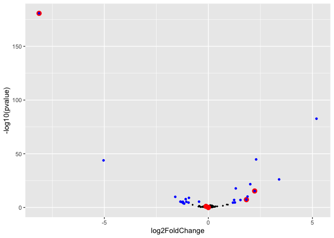
In this plot genes significantly differentially expressed are shown in
blue. Those annotated with the GO term “<GO:0032731>” are shown in red.
A negative fold change value means the gene is expressed at lower levels
in NNN mice.