BC3203

Week 8 Coding Lecture

Summarising genes in a gff file

First download some gene annotations to work with. This includes;

The yeast genome

mkdir example_data

wget ftp://ftp.ncbi.nlm.nih.gov/genomes/all/GCF/000/146/045/GCF_000146045.2_R64/GCF_000146045.2_R64_genomic.gff.gz -O example_data/yeast.gff.gz

cd example_data/
gunzip yeast.gff.gz

The fruit fly genome

wget ftp://ftp.ncbi.nlm.nih.gov/genomes/all/GCF/000/001/215/GCF_000001215.4_Release_6_plus_ISO1_MT/GCF_000001215.4_Release_6_plus_ISO1_MT_genomic.gff.gz -O example_data/dmel.gff.gz

cd example_data/
gunzip dmel.gff.gz

The Human genome

wget ftp://ftp.ncbi.nlm.nih.gov/genomes/all/GCF/000/001/405/GCF_000001405.38_GRCh38.p12/GCF_000001405.38_GRCh38.p12_genomic.gff.gz -O example_data/human.gff.gz

cd example_data/
gunzip human.gff.gz

These are gff files. They are essentially tabular but have a few header lines at the top. Look at the top of one to see

head example_data/yeast.gff

## ##gff-version 3
## #!gff-spec-version 1.21
## #!processor NCBI annotwriter
## #!genome-build R64
## #!genome-build-accession NCBI_Assembly:GCF_000146045.2
## #!annotation-source SGD R64-2-1
## ##sequence-region NC_001133.9 1 230218
## ##species https://www.ncbi.nlm.nih.gov/Taxonomy/Browser/wwwtax.cgi?id=559292
## NC_001133.9  RefSeq  region  1   230218  .   +   .   ID=NC_001133.9:1..230218;Dbxref=taxon:559292;Name=I;chromosome=I;gbkey=Src;genome=chromosome;mol_type=genomic DNA;strain=S288C
## NC_001133.9  RefSeq  telomere    1   801 .   -   .   ID=id-NC_001133.9:1..801;Dbxref=SGD:S000028862;Note=TEL01L%3B Telomeric region on the left arm of Chromosome I%3B composed of an X element core sequence%2C X element combinatorial repeats%2C and a short terminal stretch of telomeric repeats;gbkey=telomere

The third column contains the feature type. Let’s generate a list of all possible types

cat example_data/yeast.gff | awk '{print $3}' | head

## 
## 
## annotwriter
## 
## 
## R64-2-1
## 1
## 
## region
## telomere

The comment lines start with #. These are causing problems with our attempt to get the third column using awk. We can use grep to remove them.

cat example_data/yeast.gff | grep -v '^#' | awk '{print $3}' | head

## region
## telomere
## origin_of_replication
## gene
## mRNA
## exon
## CDS
## gene
## mRNA
## exon

Note the use of the regular expression anchor character, ^ this ensures that the match only occurs at the start of the line

Alternatively we could use an awk pattern to accomplish the same thing

cat example_data/yeast.gff | awk '!/^#/{print $3}' | head

## region
## telomere
## origin_of_replication
## gene
## mRNA
## exon
## CDS
## gene
## mRNA
## exon

Here we use the pattern ^# to match lines starting with # and used the negation operator, ! to invert the match (ie show lines that don’t match this pattern). In this case ! serves the same function as the option, -v that we used for grep.

Finally we can list all unique genomic feature types by using the combination of utilities sort and uniq. The uniq command will remove duplicate lines from its input but (importantly) this only works if the input is first sorted. We therefore almost always use uniq in combination with sort. By using the -c option to uniq we also get the count of the number of occurrences of each feature type.

cat example_data/yeast.gff | awk '!/^#/{print $3}' | sort | uniq -c

##       2 antisense_RNA
##    6366 CDS
##      64 centromere
##    6760 exon
##    6427 gene
##     383 long_terminal_repeat
##      50 mobile_genetic_element
##    5995 mRNA
##      14 ncRNA
##     360 origin_of_replication
##      18 pseudogene
##      17 region
##       1 RNase_MRP_RNA
##       1 RNase_P_RNA
##      14 rRNA
##      14 sequence_feature
##      76 snoRNA
##       6 snRNA
##       1 SRP_RNA
##       1 telomerase_RNA
##      32 telomere
##      10 transcript
##     299 tRNA

As this is a very well studied genome it contains a range of interesting feature types not found in draft genomes such as the origin of replication, centromere, telomere and many different types of RNA. Most commonly we are just interested in the genes. There are several gene related entries because genes are actually fairly complex genomic features. For a complete description of how genes are represented in gff see this page from the gene ontology consortium. For our purposes we will just consider the following gene related feature types;

Feature Name	Description
`gene`	Describes the boundaries (start and stop) of the entire gene
`mRNA`	Describes the boundaries of the mRNA products of the gene
`exon`	A portion of a gene that is incorporated into at least one mRNA
`CDS`	CoDing Sequence. Portion of an exon that actually codes for protein

Our goal will be to summarise each gene by its length and the number of alternative mRNA that it encodes. This is a feature that varies considerably between organisms such as yeast and higher eukaryotes such as fruit flies.

Using Tidyverse to read and summarise gffs

library(tidyverse)
dmel_gff <- read_tsv("example_data/dmel.gff", 
                     comment="#",
                     col_names = c("seqid","source","type","start","end","score","strand","phase","attributes"),
                     col_types = cols())

Let’s start by summarising the gene density along several chromosomes.

To do this we first need to download chromosome info for Dmel

wget 'https://bc3203.s3.ap-southeast-2.amazonaws.com/lecture14/dmel_chroms.xlsx' -O example_data/dmel_chroms.xlsx

## --2021-09-13 01:02:07--  https://bc3203.s3.ap-southeast-2.amazonaws.com/lecture14/dmel_chroms.xlsx
## Resolving bc3203.s3.ap-southeast-2.amazonaws.com (bc3203.s3.ap-southeast-2.amazonaws.com)... 52.95.132.51
## Connecting to bc3203.s3.ap-southeast-2.amazonaws.com (bc3203.s3.ap-southeast-2.amazonaws.com)|52.95.132.51|:443... connected.
## HTTP request sent, awaiting response... 200 OK
## Length: 11730 (11K) [application/vnd.openxmlformats-officedocument.spreadsheetml.sheet]
## Saving to: 'example_data/dmel_chroms.xlsx’
## 
##      0K .......... .                                          100% 32.0M=0s
## 
## 2021-09-13 01:02:07 (32.0 MB/s) - 'example_data/dmel_chroms.xlsx’ saved [11730/11730]

dmel_chroms <- readxl::read_excel("example_data/dmel_chroms.xlsx")

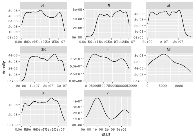
We then join the Chromosome info with the gff file and plot density along named chromosomes only

dmel_gff %>% filter(type=="gene") %>% 
  left_join(dmel_chroms,by=c("seqid"="RefSeq")) %>% 
  filter(!is.na(Name)) %>% 
  ggplot(aes(x=start)) + 
  geom_density() +
  facet_wrap(~Name, scales = "free")

Our next goal is to summarise the number of isoforms for each gene as well as the length of each gene. To do this we need to create two new columns;

A geneid which needs to be extracted from attributes
gene length which is easily calculated from (end-start)

dmel_gene_rna <- dmel_gff %>% 
  filter(type %in% c("gene","mRNA")) %>% 
  tidyr::extract(attributes,into = "geneid" ,regex = "GeneID:([0-9]*)") %>% 
  mutate(feature_length = end-start)

dmel_rna_gene_len <- dmel_gene_rna %>% 
  group_by(geneid) %>% 
  summarise(num_isoforms=n()-1, gene_length = max(feature_length)) 

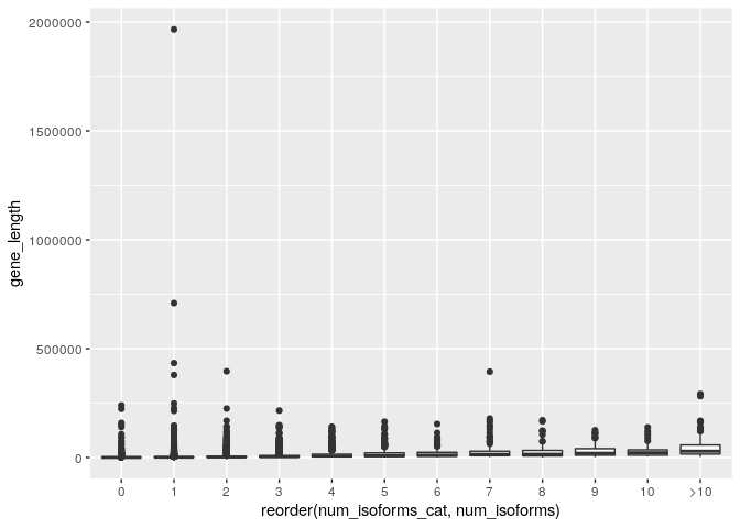
ggplot(dmel_rna_gene_len,aes(x=gene_length,y=num_isoforms)) + geom_point()

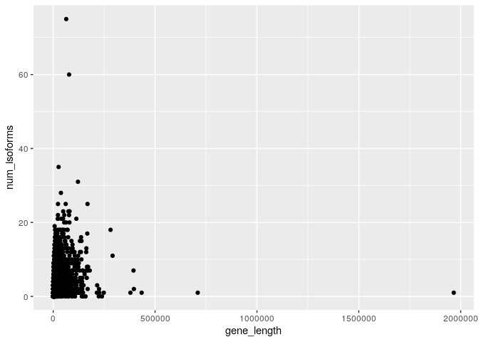
This plot is extremely ineffective for several reasons;

It seems to be driven by a handful of extremely unusual genes. For example the fruit fly gene gene13246 is almost 2Mb in size. This is actually a real gene and codes for the protein, Myosin 81F.
There are many points plotted over the top of each other so that most of the useful information in the data is obscured

To solve these problems let’s try making num_isoforms into a categorical variable. In order to do this let’s first make a histogram of num_isoforms to see the spread of its values

ggplot(dmel_rna_gene_len) + geom_histogram(aes(x=num_isoforms), binwidth = 1) + xlim(0,20)

## Warning: Removed 19 rows containing non-finite values (stat_bin).

## Warning: Removed 2 rows containing missing values (geom_bar).

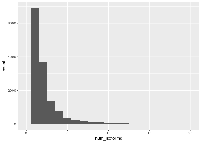
This suggests that it might be sensible to use the num_isoforms variable as-is but with all genes with say >10 isoforms lumped into a single category.

gene_data_cat <- dmel_rna_gene_len %>% 
  mutate(num_isoforms_cat = ifelse( num_isoforms <= 10, as.character(num_isoforms), '>10'))

Now use a boxplot to summarise the relationship

ggplot(gene_data_cat) + geom_boxplot(aes(x=reorder(num_isoforms_cat,num_isoforms), y=gene_length))

Again this is not very good because the distribution of gene lengths seems to have many large outliers but is concentrated at low values. This suggests that it may be log-normally distributed. A fix would therefore be to log transform the length scale

ggplot(gene_data_cat) + geom_boxplot(aes(x=reorder(num_isoforms_cat,num_isoforms), y=log(gene_length)))

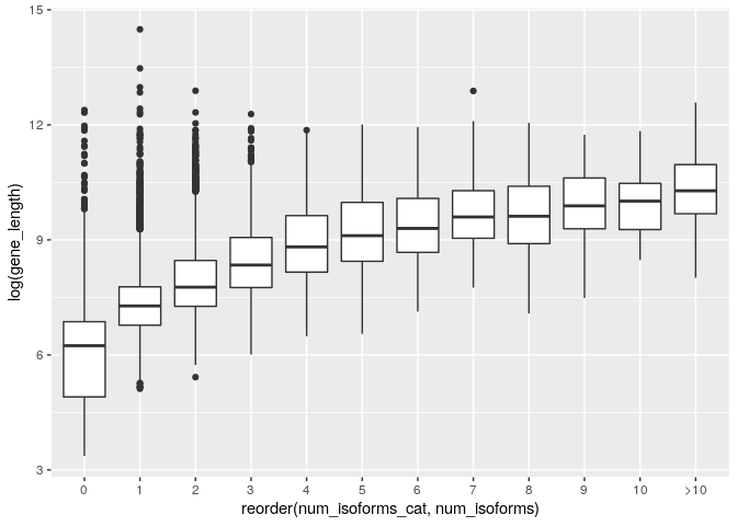
This is much better. It shows that although there are some very long genes with few isoforms the general trend is for genes with more isoforms to be longer.

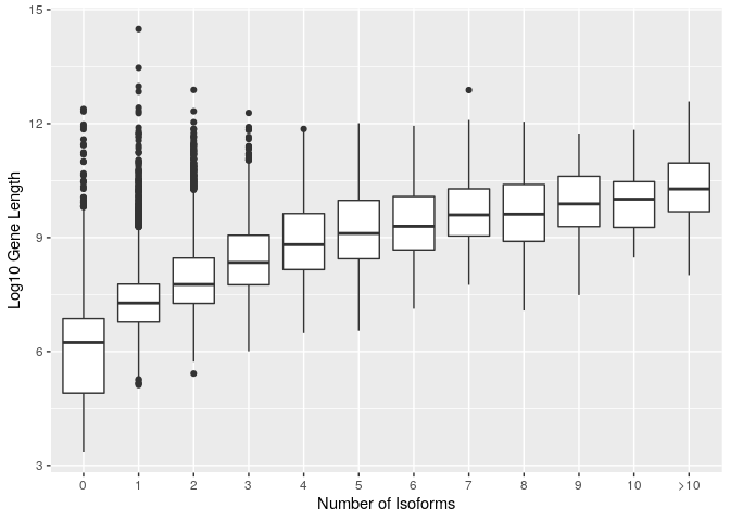
Finally we clean up the axis labels

ggplot(gene_data_cat) + 
  geom_boxplot(aes(x=reorder(num_isoforms_cat,num_isoforms), y=log(gene_length))) +
  xlab("Number of Isoforms") +
  ylab("Log10 Gene Length")

Dealing with multiple species

Now let’s consider how to compare the relationship between number of isoforms for different species. We have three species, Human, Yeast and Drosophila.

Most of the data wrangling steps we used for Dmel can be applied as-is for the other species. This suggests that we should create a function to perform these steps. We do this using a series of functions as follows;

First the gff reading step

read_gff <- function(gff_path){
  read_tsv(gff_path, 
           comment="#",
           col_names = c("seqid","source","type","start","end","score","strand","phase","attributes"),
           col_types = cols())
}

dmel_gff <- read_gff("example_data/dmel.gff") %>% add_column(species="dmel")
human_gff <- read_gff("example_data/human.gff") %>% add_column(species="human")
yeast_gff <- read_gff("example_data/yeast.gff") %>% add_column(species="yeast")

Now we can simply concatenate all these gff files together end-to-end with rbind

all_species_gff <- rbind(dmel_gff,human_gff,yeast_gff)

The geneid parsing, isoform counting, and categorisation can be done as before but this time we group_by species and geneid

all_species_gff_rna_cat <- all_species_gff %>% 
  filter(type %in% c("gene","mRNA")) %>% 
  extract(attributes,into = "geneid" ,regex = "GeneID:([0-9]*)") %>%
  mutate(feature_length = end-start)  %>% 
  group_by(geneid,species) %>% 
  summarise(num_isoforms=n()-1, gene_length = max(feature_length)) %>% 
  mutate(num_isoforms_cat = ifelse( num_isoforms <= 10, as.character(num_isoforms), '>10'))

## `summarise()` has grouped output by 'geneid'. You can override using the `.groups` argument.

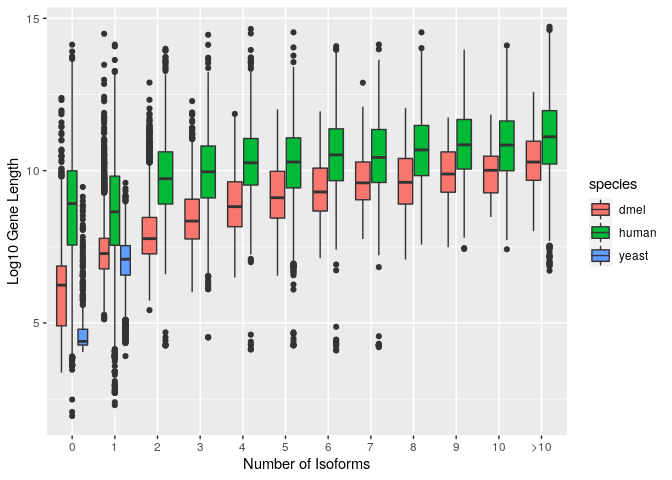
This allows us to make a plot by species

ggplot(all_species_gff_rna_cat) + 
  geom_boxplot(aes(x=reorder(num_isoforms_cat,num_isoforms), y=log(gene_length),fill=species)) +
  xlab("Number of Isoforms") +
  ylab("Log10 Gene Length")