BC3203
Tutorial 2 : Variables, Loops and Permissions
Goal
This tutorial has several goals;
- Extend your unix command line skills beyond those learned in Tutorial 1
- Provide hands on experience cleaning and assessing the quality of real sequencing data
Assumed Knowledge
This tutorial assumes that you have some basic knowledge of using the unix command line. Before you start you should therefore make sure that you have completed;
- The interactive tutorial which covers basic unix commands;
- Coding assignment 1 ( see https://bc3203.bioinformatics.guide for links to the guide and exercises)
Setup
Setup RStudio to work with a clone of this repository. To do this you will first need to setup your github account and SSH keys as explained in the guide to tutorial 1.
If you have already completed tutorial 1 you can go directly to the following
- Accept the assignment on github classrooms using this link
- Navigate to your copy of the assignment on github and obtain the URL to “Clone or Download” the repository using SSH.
- Create a new project in RStudio using version control and add the URL from step 2.
All these steps are explained in more detail in the guide to tutorial 1
How to complete this tutorial
Start by reading the this document (you are in the right place). Do the exercises when instructed.
The assessable component is contained within the file exercises.Rmd. Open this file by clicking on it in RStudio. This is where you should enter answers to your questions. Your mark for this tutorial will be obtained from your answers to questions in this file.
You might also want to create a new RMarkdown document where you can practise commands. Give it a name that makes it clear that this is not your final answers (eg exploration.Rmd or practise.Rmd). Running practise code is a very important part of the learning process. You should feel free to add practise code to this file or to simply run it in a Terminal window. Important This file is for practising only. We will ignore everything in this file when marking assignments.
Optional: A guided walkthrough of analyzing sequencing data for quality control issues (see last section of this page). This is not required for assessment purposes but will be useful to help understand concepts taught in lectures and which might form part of questions on the exam.
Background Information
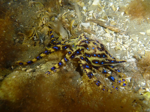
In this tutorial we will be working with a subsample of real data from a paper that sequenced the transcriptome of the Blue Ringed Octopus (Hapalochlaena maculosa) from multiple body tissues. The study was part of a project to sequence the Blue Ringed Octopus genome that was published in gigascience in 2020. The project was led by PhD student, Brooke Whitelaw within the Marine Omics research group at JCU.
This tutorial closely mirrors a process that is often required to download data provided by a sequencing centre. It also introduces general concepts (loops and variables) that are useful in many contexts when working with large numbers of input files.
Part 1: Downloading and Securing Data
Good News!
The sequencing center has just sent you an email to tell you that the data is ready. In their email they tell you that there are 24 separate files available for download. It would be slow and error prone to individually download them but fortunately the file names and the URLs for download follow a pattern. This will allow us to automate the process. In real projects it is common to work with hundreds or even thousands of sequencing input files so performing operations without automation is simply not an option.
The sequencing center tells you that the download URLs look like this
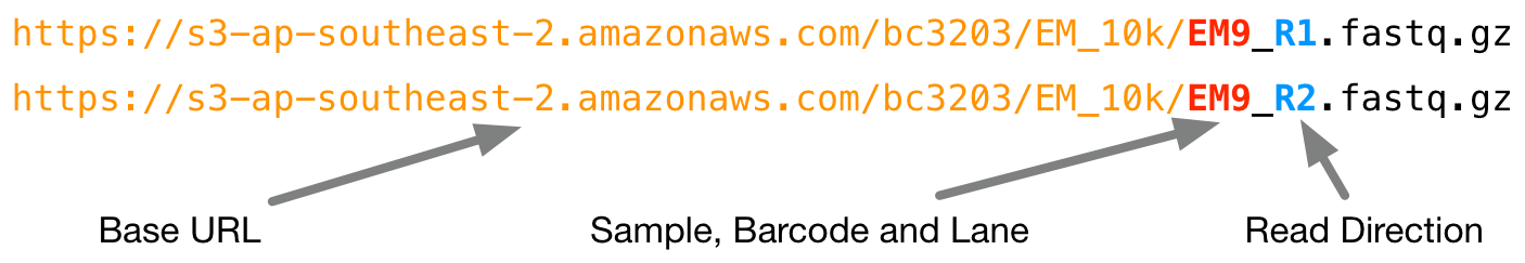
When you submitted samples to the sequencing center you provided sample codes for each of twelve tissues in a single animal (see table below). Paired end sequencing was used so there will be two files for each sample, an R1 file corresponding to forward reads and an R2 file corresponding to reverse reads.
| Sample Code | Tissue |
|---|---|
| EM1 | skin dorsal mantle |
| EM2 | eyeballs |
| EM3 | gills (plus branchial gland) |
| EM4 | Branchial Hearts |
| EM5 | Renal appendages |
| EM6 | systemic heart |
| EM7 | Male Reproductive tract (immature) |
| EM8 | Posterior salivary glands |
| EM9 | Ventral mantle muscle (plus skin) |
| EM10 | Brain |
| EM11 | Anterior salivary glands |
| EM12 | Digestive Gland |
Your task will be to create a small script to download all the data. This task will require you to learn several new concepts. We will build these in steps.
Variables
Variables are placeholders for information. They occur in all programming languages including bash. For example we could make a variable called sample and assign its value to one of our sample names like this;
sample="EM1"
If we ever want to get that information back we can use the $ operator to retrieve it as follows;
sample="EM1"
echo $sample
Note that since the RStudio bash interpreter gets started fresh for every code block it can’t remember variables from block to block. This works differently when you work directly in the Terminal. Each terminal session will remember all the variables you enter until you close that terminal window or logout.
The echo command also allows you to mix variables and fixed strings together for example
sample="EM1"
echo $sample
echo "${sample}_R1.fastq.gz"
Note the use of curly brackets around the variable in the second example (ie ${sample}). These are required because without them the interpreter would not know which part of the string is our variable and which is normal text.
Notice how the last command here substitutes the content of ${sample} into the appropriate place within a larger string. This is extremely useful for automation because the same code can generate different strings depending on the value we store in the variable ${sample}. For example;
sample="EM1"

echo "${sample}.fastq.gz"

sample="EM2"

echo "${sample}.fastq.gz"
And so on …
But this still isn’t very useful is it? What if we could automate the process of assigning a new value to sample so that it went through all the samples in our list of 12 samples. Now that would be useful!
This is where the concept of a loop comes in.
Loops
Loops allow you to perform the same task repeatedly in different contexts (eg on different files, different names in a list, columns in a table etc etc)
Most programming languages support looping in some form or another. The syntax for a for loop in bash is like this
for placeholder in <list>
do
  <commands>
done
This will take each item in <list> and temporarily assign it to a variable called placeholder. The part between do and done can include as many commands as we want and we can refer to the current value of placeholder when running commands. For example we could do the following;
for sample in EM1 EM2
do
  echo "${sample}.fastq.gz"
done
Run this code by pasting it into Terminal. The output should look familiar. Using a loop we have now accomplished the same thing as we did above by typing out the echo command multiple times.
Before you move on to answer questions 1 and 2 try playing around with this example loop.
- What happens if you change the name of the placeholder variable?
- What happens if you change the list items? Try adding some more.
- What happens if you add more or different commands in the space between
doanddone?
Stop: Answer questions 1 and 2 in the exercises before reading further
Generating a sequence
In the for loops above we had to laboriously type out all the sample names, “EM1”, “EM2”, “EM3” … and so on. This type of repetitive pattern is exactly the sort of thing that can be easily automated. In this case we simply have a sequence of sample codes numbered 1 through to 12 with “EM” prepended to each.
The seq command in bash can be used to generate a sequence of numbers. For example;
seq 1 3
Capturing the output of a command
Most of the time when you run a command its output is simply printed to the screen. Previously we’ve seen that output redirection can be used to send this output to a file (ie using > and >>). Alternatively, outputs can be captured in a variable.
This is done using the following syntax
variable=$(<command>)
numbers=$(seq 1 3)
echo $numbers
Captured output can be used to generate a list for looping, like this
for num in $(seq 1 3)
do
  echo "num is $num"
done
Stop: Answer questions 3-5 in the exercises before reading further
Downloading files
The wget command is a very powerful way to download files. It supports a wide range of internet protocols, methods of authentication and allows alot of things to be customized about how it does its job. Just to get some idea of how powerful this command is try looking at its manual page;
man wget
Another program that can also be used for this purpose (and others) is curl.
We will use wget to download our sequencing files. Since there a lot of files we should organise them into a separate directory.
We put them into data/sequencing
mkdir -p data/sequencing
Now try downloading a single file with the following command
wget https://s3-ap-southeast-2.amazonaws.com/bc3203/EM_10k/EM10_R1.fastq.gz -O data/sequencing/EM10_R1.fastq.gz
Note the use of -O to specify the path to the output file. Without this option the file would be saved to the current working directory.
After running the command use the RStudio file browser to verify that the file actually downloaded.
Stop: Answer questions 6-7 in the exercises before reading further
Securing Data
Sequencing data is often expensive and time consuming to generate. As you progress with your analyses you will generate a lot of “derived” data which represents the results of analyses you perform. Using tools like RMarkdown and running as many analyses as possible on the command line mean that these “derived” datasets can often be regenerated relatively easily. The raw sequencing data on the other hand cannot be regenerated.
After downloading raw data you should always make it “read only”. This protects the data against you accidentally overwriting it or using the rm command to delete it. It isn’t total protection (please also have a backup) but it is a basic first step.
All files in unix are associated with a set of permission information. This image provides a brief summary
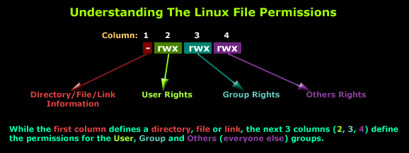
The permissions for a file can be viewed with the ls command by using the -l option. For example we can view permissions for one of our downloaded files as follows;
ls -l data/sequencing/EM1_R1.fastq.gz
Inspect the results of this ls command. Most likely you will see that the user (you) has both r (read) and write w permissions. Other users in the same group can read and everyone else can read. You might also see other symbols like @. These represent extended attributes of the file beyond the usual unix standard (these are common on macOS and are used to support macOS specific features like sandboxing). Don’t worry about these for now.
The chmod command can be used to change permissions on a file. An easy way to use chmod is with the following syntax
chmod <ugo><+-><rwx> file
- The first part
ugospecifies who is affected (ie user, group, other). Multiple selections are allowed egug(modify permissions for user and group) - The second part
+-says whether we will be adding+or removing-permissions - The last part specifies the permissions to add or remove.
For example we could remove write and execute permission for all users (making a file readonly) as follows;
chmod ugo-w data/sequencing/EM1_R1.fastq.gz
ls -l data/sequencing/EM1_R1.fastq.gz
Stop: Answer questions 8 and 9 in the exercises
Sequencing Quality Control with FastQC
For almost any sequencing project the first thing you should do after downloading files is to check quality metrics. The mostly widely used tool for this purpose is a command-line program called fastqc
Sequencing Data
To give you an idea of what to expect from different platforms we have prepared a set of example data which includes a range of sequencing projects (The Blue Ringed Octopus transcriptome is included). The examples are;
| File | Details |
|---|---|
| 16s_300bp_pe_miseq | Coral Microbiome data from the JCU MiSeq |
| wgs_100bp_pe_hiseq_100k | Whole genome resequencing data of Acropora tenuis from Magnetic Island |
| EM10 | Blue Ringed Octopus Brain transcriptome. |
All the data were sequenced with Illumina technology but they encompass a wide range of applications including 16S microbiome, whole genome sequencing (wgs) and whole transcriptome sequencing.
Download the example data using wget and save it to your data folder as follows;
wget https://s3-ap-southeast-2.amazonaws.com/bc3203/fastqc_examples.tar.gz -O data/fastqc_examples.tar.gz
Note: This is a sizeable download so you may need to wait a few minutes.
The examples are packaged into a single file with the extension tar.gz. tar stands for tape archive and is a standard way to package up multiple files and directories into a single file. The .gz extension denotes that this tar file is gzipped (compressed).
Use the tar command to unpack the file;
cd data
tar -zxvf fastqc_examples.tar.gz
Note that this example uses several options stuck together. Specifically -z tells tar to unzip the archive, -x tells it to extract it, -f tells it to expect a file as input and -v tells it to print verbose output (so we can watch progress).
After unpacking the file move back up to the top level of your tutorial directory. The commands that follow assume that this is where you are or that you run commands from within an RMarkdown code block.
cd ../
FastQC
To view the help for fastqc run it with -h
fastqc -h
Now try running fastqc on a single file. Start with the smallest since this will run nice and quick
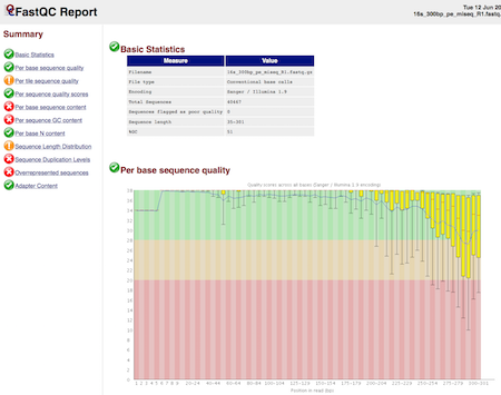
fastqc data/fastqc_examples/16s_300bp_pe_miseq_R1.fastq.gz
When this command finishes it should create two new files inside data/fastqc_examples. The most interesting file is the one with a .html extension. In RStudio you should be able to click on this file and select Open in Browser to view it. It should look like this
Now run fastqc on all the remaining fastq.gz files in the fastqc_examples directory.
fastqc data/fastqc_examples/*.fastq.gz
Explore the results by opening the .html files. Look at all the results but focus on the things that fail QC. In some cases fastqc flags a failure even when this is just “normal” for the application. Use articles on qcfail and from this webpage on RNAseq specific failures to help you interpret the results for each dataset.
Some specific things to think about
-
The
16Smicrobiome dataset consists of the same gene amplified in many different organisms. Many of the DNA fragments being sequenced will therefore be very similar. How might this affect the results for the16SQC? -
The
EM10sample includes a file with 100 thousand reads. Compare the results you got from this file with the result in the folderprecalcwhich are for the entire dataset (24 million reads). Notice that the full dataset includes a warning about sequence duplication levels. Why might this be expected if the read depth is increased? In the sequence duplication plot you will see a peak at high duplication levels (>10) indicating that there is a subset of reads that are highly duplicated whereas most are not. How does this reconcile with what you know about RNA?