BC3203
This dataset comes from a study by JCU PhD student, Jia Zhang. The goal of that study was to understand the evolutionary origins of “super” tough corals inhabiting reefs in the Kimberley region of Western Australia. To do this, genetic variants of the coral, Acropora digitifera, were analysed based on samples from the Kimberley, Rowley Shoals and Ashmore Reef. The overall hypothesis of the study is that corals in the Kimberley should harbour genetic differences from offshore reefs (Rowley Shoals, Ashmore Reef) that allow them to survive extremes of temperature, long intertidal exposure times, and highly variable turbidity.
The work was published in 2022 in the journal Molecular Biology and Evolution. Note that the analyses in this study are very extensive and many involve specialist population genetics knowledge which we have not covered in this subject. You are by no means expected to reproduce these analyses. You do not need a background in genetics to complete this assignment but if you do have such a background you should feel free to use your knowledge to extend the scope of work to include whatever analyses you feel would be appropriate.
Data Setup
The data for this assignment is located at the path /pvol/data/coralvar on the class rstudio server. Run the following commands to create a symbolic link to this in the data directory of your assignment
cd data
ln -s /pvol/data/coralvar .
The following files are present within the coralvar data directory;
| File Name | Purpose |
|---|---|
metadata.tsv |
A tab separated values file with information on the sampling locations for each coral colony in the study |
*.bam |
Sequence alignment data. Each .bam file represents paired-end Illumina sequencing reads that have been aligned to the Acropora digitifera genome for a single coral colony. Sample IDs are encoded in the filenames of these *.bam files. |
GCA_014634065.1_Adig_2.0_genomic.fna |
The full genomic sequence of Acropora digitifera |
genes.gff |
Gene models for the Acropora digitifera genome |
western_australia |
Folder containing map data for the WA coastline |
Key software tools
- bcftools for variant calling and filtering
- vcftools for variant filtering and some genetic analyses
- plink2 for calculating genetic PCA and Fst
- IGV for visualising overlap of genes with SNPs
- bedtools for finding genes that overlap with SNPs
awkfor filtering and transforming tables of values
Visualising Sample Locations
There are many excellent options for making publication-quality maps in R. The simple features package is particularly easy to use as it provides extensions to ggplot2 for map layers. The code below provides a bare bones illustration of how you might use this package to plot the sampling locations from this study.
library(sf)
library(tidyverse)

wa_coast <- st_read("data/coralvar/western_australia/",layer = "cstwacd_l") %>%
  filter(FEAT_CODE=="coastline")

wa_coast_cropped <- st_crop(wa_coast, xmin = 113.8, ymin = -22.59, xmax = 128.51, ymax = -6.49)

projcrs <- "+proj=longlat +datum=WGS84 +no_defs +ellps=WGS84 +towgs84=0,0,0"

site_summaries <- read_tsv("data/coralvar/metadata.tsv") %>%
  group_by(site_name,lat,lon) %>%
  summarise(n_samples=n())

sites_sf <- st_as_sf(site_summaries,coords = c("lon", "lat"),crs = projcrs)

ggplot() +
  geom_sf(data=wa_coast_cropped) +
  geom_sf(data=sites_sf, lwd=1,aes(color=site_name,size=n_samples)) +
  theme_bw()
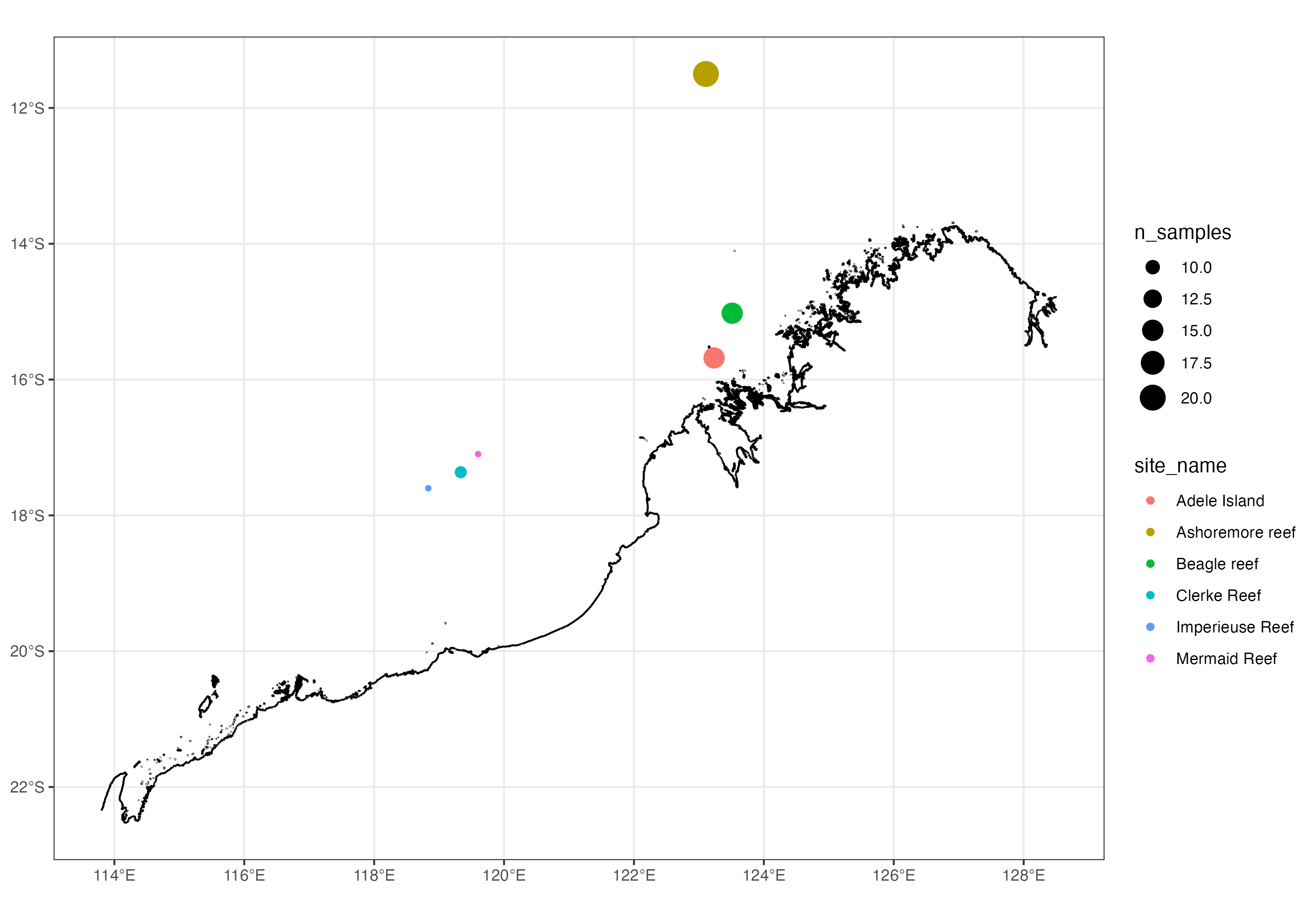
Map of the Western Australian coastline showing sampling locations used in this study
Germline Variant Calling
The full dataset for this paper is very large as it represents the whole genomes of 75 coral colonies, each of which was sequenced to a depth of around 20x. To make things tractable for this assignment the data has been trimmed down to represent just a few thousand variable sites across the genome. Nevertheless, even with this trimmed data a vast array of analyses are possible.
Regardless of what else you plan to do with this data you will almost certainly want to begin by performing germline variant calling. This topic was covered in Matt Field’s lectures and you will have encountered it in a human context in the variants coding assignment.
Rather than using the GATK variant caller we will use the bcftools variant caller as this is faster and simpler. To call variants you will need the reference genome, GCA_014634065.1_Adig_2.0_genomic.fna and bam files with reads aligned to this genome. Once these are ready you can call variants with bcftools in two steps as follows (NOTE: Do not run these commands interactively. Make a slurm script to run them in the background and include this slurm script in the github repository for your assignment).
bcftools mpileup -q 20 -Q 20 -f GCA_014634065.1_Adig_2.0_genomic.fna *.bam -Ob > tmp.mpileup
This first step produces an mpileup file which is essentially a summary of evidence for variants at each position in the genome (ie how the reads are piled up against the genome). Next we use this as input to bcftools call to actually call the variants.
bcftools call -v -Ov -o coral.vcf -m tmp.mpileup
Finally. Delete the mpileup file as this is not needed and is a waste of disk space
rm tmp.mpileup
Basic Variant Filtering
After performing variant calling you should have a vcf file with several hundred thousand variants. You can count the number of variants in the file as follows;
bcftools view -H coral.vcf | wc -l
Many of these variants will be low quality (possibly false positives) that we would like to remove from our analyses. Variant filtering is a complex topic that we have not covered fully in this subject. For the purposes of this assignment just perform some basic cleanup. We do this in a series of steps. At each step we produce a new vcf file and will check it to see how many variants were retained
- Remove variants supported by just a single alternate allele (minor allele count of less than 2)
vcftools --vcf coral.vcf --mac 2 --stdout --recode --recode-INFO-all > coral1.vcf - Remove sites with very low or very high read depth. In this dataset we have 75 samples and would like to exclude any sites where the mean depth is 10x or less (total depth <750) and where the depth is greater than 33x (>2500). Both low and high depth sites can be a sign of poor mapping quality.
bcftools filter -e 'DP<750 || DP>2500' coral1.vcf > coral2.vcf - Remove sites with more than 10% missing genotypes and keep only biallelic SNPs
vcftools --vcf coral2.vcf --max-missing 0.9 --min-alleles 2 --max-alleles 2 --remove-indels --stdout --recode --recode-INFO-all > coral3.vcf
Suggested Analyses
Once you have completed variant calling you should have a vcf file. This can be used to perform many analyses using programs installed on our rstudio server such as vcftools and plink.
Principle Components Analysis (PCA). A genetic PCA using the vcf file can be used to reveal distinct groupings or clusters of samples (AKA genetic structure). A simple way to perform the PCA is using plink2 as follows
plink2 --vcf coral3.vcf --out adig --pca --allow-extra-chr
After running this command you will have a pair of output files *.eigenvec and *.eigenval. The eigenvec file contains the position of each sample within the multidimensional space of the PCA. Here you are most likely only interested in plotting samples in 2 dimensional space (PC1 vs PC2). The values in the eigenval file provide the relative amounts of variation explained by each of the PC axes.
Pairwise Fst for each variant site. Fst measures the degree to which frequencies of alleles differ between groups of individuals (populations). In your PCA (step 1) you should be able to identify genetically distinct groups of individuals. Now you can calculate the Fst between each pair of groups. Essentially Fst measures the degree to which individual genomic loci have diverged between populations. A value of 1.0 indicates that a variant is completely fixed in one population and absent in another (ie total differentiation) whereas a value of 0 indicates no differentiation (equal variant frequencies in the two populations). We expect some differentiation to occur over time in all sites due to neutral processes such as genetic drift. If natural selection has acted to increase the fequency of specific alleles in certain populations we may see extremely high or “outlying” values of Fst at specific sites.
To prepare data for calculating Fst with plink you will need to prepare a text file in which each individual sample is listed in the first column and the grouping to which that sample is assigned is listed in the second column. For example the top few lines of your file should look something like this
  #IID  site
  AI_1_001_S102_L004	inshore
  AI_1_008_merged	inshore
  AI_1_021_S97_L004	inshore
Assuming you have you named this file populations.txt you can now calculate Fst for each pair of populations and for every variant locus as follows;
plink2 --fst site report-variants --pheno populations.txt --vcf coral3.vcf --allow-extra-chr
This will produce several output files as follows;
| File Name | Purpose |
|---|---|
| plink2.pop1.pop2.fst.var | Fst values for individual SNPs between pop1 and pop2. There should be 3 such files if you had three genetic groupings |
| plink2.fst.summary | Average Fst value (across all sites) for each pair of populations. |
Examine the Fst results carefully. Is there one population that seems more divergent than the others? Do you see any SNPs with an unusually high value of Fst? If so, what can you say about the genomic region(s) where these high values are found? Do they overlap with known genes?
To investigate these questions you should load Fst values into R and explore the distribution of values. To find out whether SNPs overlap with genes you can load both SNPs and gene models into a genome browser such as IGV or use bedtools.