BM3331 / BC5203
Background
In this tutorial we will work with a gff (General Feature Format) file containing the locations of all the features (genes, exons, introns etc) on the human genome.
The guide for this tutorial provides instructions on command-line (BASH) code that you will need to run in order to generate datasets required for further processing with R. This reflects the reality of many bioinformatic workflows. Often we will start by using command-line tools to cut datasets down to a manageable size, or perform resource intensive tasks. We will then export data to a form that can be read into R and used for visualisation or further analysis.
Setup
Setup RStudio to work with a clone of this repository and make sure you understand how to submit your edits so that they can be graded. This is all explained in the guide to tutorial 1.
Next, run the setup code. This will download and unpack example data used for this guide, and for the corresponding exercises.
bash setup.sh
After running the setup code you should see the following files in your data folder;
| Name | Description |
|---|---|
GCF_000001405.39_GRCh38.p13_genomic.gff |
Human genome annotations |
Chromosomes.xlsx |
Human chromosome information |
Several questions in the exercises ask you to write code that produces a plot. Look carefully at the expected plots. Details like axis labels, legend titles and scales should all be the same, because the automated tests only pass if your plot is essentially identical to the expected one. Other questions ask you to write a function or produce a table. You can view the expected outputs for all questions at https://bc3203.bioinformatics.guide/2026/tutorials/06/expected_outputs
Each question is tested on its own, so each answer must include all the code it needs. The exercises explain this in more detail.
Features in the Human Genome
Take a look at the NCBI RefSeq page for the Human Genome. The annotation file we will use comes from an earlier release of this genome (GRCh38.p13), but its format is the same. This page provides a summary of the genome sequence as well as its annotation (ie inferences about where the genes are). Tools are provided via this page for downloading various files associated with the genome and its annotation. There are quite a few different files associated with a Genome for an organism. There are two main types;
- Sequences in FASTA format. This includes;
- genome: the actual sequences for each chromosome and mitochondrion
- transcript: sequences for all the individual mRNAs corresponding to genes
- protein: translations of all the mRNA sequences
- Annotations. These are the positions (start, end) and descriptions of all the features (chromosomes, genes, exons, introns, coding sequences etc) in the genome. The positions given refer to a given sequence entry in the genome file (eg a chromosome) and the number of bases along that sequence where the feature exists.
In this tutorial we will focus on the annotation file in gff format. It’s just a simple tabular format. There are 9 fields separated by tab characters. These are effectively “columns” in a table of data. The fields (columns) we are most interested in for now are just the first 5;
| Field | Description |
|---|---|
| seqid | name of the chromosome or scaffold |
| source | name of the program that generated this feature, or the data source (database or project name) |
| type | feature type name, e.g. gene, exon, CDS |
| start | Start position of the feature, with sequence numbering starting at 1 |
| end | End position of the feature, with sequence numbering starting at 1 |
The remaining four fields are score, strand, phase and attributes. We will look at attributes later in this guide.
Use the command below to inspect the first few lines of the gff file. This command uses head to obtain the first few lines and cut to restrict the output to columns 1-5
head data/GCF_000001405.39_GRCh38.p13_genomic.gff | cut -f1-5
Notice that the first 9 lines are not part of the table. They all start with a # and provide some overall metadata about the whole file. Next count the total number of lines in the file to get an appreciation for how large it is;
wc -l data/GCF_000001405.39_GRCh38.p13_genomic.gff
We would like to read the file into R to work with it but it is nearly 3.9 million lines long. It’s certainly possible to read a file this big into R, but it will take a long time and use a lot of memory. Next, we will use a tool called grep and another called awk to cut the file down to size so that we can work with only the relevant parts of it in R.
Unix Text Utilities
The unix text processing utilities, awk, sed and grep are incredibly useful tools for transforming biological data. By combining these three utilities with other standard unix tools such as cat, sort, uniq and wc we can accomplish almost any kind of text processing on the command-line.
Rather than trying to learn all these tools in one go we will encounter them gradually and learn them in the context of tasks we want to accomplish.
Recall from the gff format definition that the third column denotes the feature type. What types of features are included in a gff file? We will use unix text utilities to find out.
grep
Let’s start by removing the comment lines. Most of these are at the start of the file but there are more scattered through it. We can do this using grep. At its core, grep allows you to search for patterns of text in documents.
The most common usage of grep is like this
grep <pattern> file1
So, if we wanted to filter the Human gene annotations so that they only contained the comment lines we could use this command;
head data/GCF_000001405.39_GRCh38.p13_genomic.gff | grep '^#'
Note that a comment is denoted by the symbol, # at the start of a line. The pattern used in the command above is a little more complex because it also includes the special character ^ which tells grep to look for the string at the start of the line only.
Now let’s try modifying the behaviour of grep. Try giving it the option -v as shown in the code below;
head data/GCF_000001405.39_GRCh38.p13_genomic.gff | grep -v '^#'
What’s happened here? Take a look at the manual entry for grep.
man grep
When viewing the man page you can use spacebar to scroll down, b to scroll up, and q to quit. You should be able to find an entry that explains the -v option. It says;
-v, --invert-match
       Invert the sense of matching, to select non-matching lines.
So when we used -v it excluded all of the comment lines. This is very useful because we can now process the file reliably, knowing that every line will have exactly 9 tab delimited columns
Let’s try showing a few additional lines
head -n 20 data/GCF_000001405.39_GRCh38.p13_genomic.gff | grep -v '^#'
We are only interested in the third column for now as this describes the feature type. We can extract this using cut as follows;
head -n 20 data/GCF_000001405.39_GRCh38.p13_genomic.gff | grep -v '^#' | cut -f 3
sort and uniq
The sort command can be used to sort text. The default behaviour of sort is to sort alphabetically on the first column of text but it can be used to sort numerically on specific columns.
Try using sort to arrange the feature types in alphabetical order
head -n 20 data/GCF_000001405.39_GRCh38.p13_genomic.gff | grep -v '^#' | cut -f 3 | sort
The uniq command finds unique occurrences in text and removes duplicates. In order to work properly the input to uniq must first be sorted. A very common combination of tools is therefore to pipe sort to uniq, ie sort | uniq.
Let’s try it out on the genomic features
head -n 20 data/GCF_000001405.39_GRCh38.p13_genomic.gff | grep -v '^#' | cut -f 3 | sort | uniq
Now have a look at the manual page for uniq. You should find an option -c which is described as follows
-c, --count
       prefix lines by the number of occurrences
We can use this to modify our command so that it will also include a count of the number of times each feature occurs
head -n 20 data/GCF_000001405.39_GRCh38.p13_genomic.gff | grep -v '^#' | cut -f 3 | sort | uniq -c
And finally, we can add another sort command, this time to sort numerically by the number of occurrences, putting the features with the most occurrences at the top.
head -n 20 data/GCF_000001405.39_GRCh38.p13_genomic.gff | grep -v '^#' | cut -f 3 | sort | uniq -c | sort -n -r
So far we have worked with just a tiny fraction of the feature file. This is a good way to work when you are building up a command, figuring out how to get all the pieces in place. Now that we have things working let’s apply it to the entire file. We will also pipe our final output to head so that we see the top few, most abundant features in the file
cat data/GCF_000001405.39_GRCh38.p13_genomic.gff | grep -v '^#' | cut -f 3 | sort | uniq -c | sort -n -r | head
We can see that the most common genomic features are exon, CDS, mRNA and gene in that order. Notice that there are more mRNA entries than gene entries. This is because alternative splicing can give rise to multiple mRNA entries per gene.
Our goal is to use R tidyverse functions to explore the properties of gene entries in this file. We would therefore like to create a new version of this genome annotation file that only contains entries where the third column matches the keyword gene. To accomplish this, we will introduce a new tool, called awk.
AWK
The awk command processes text line by line. The awk programming language is used to specify actions to be performed on each line.
This illustrates the general usage of awk which is
awk 'program' file
Or alternatively, when used with a pipe
cat file | awk 'program'
Where the placeholder text, ‘program’ is a small program written in the awk language. In general awk programs are organised like this;
pattern { action }
Here’s how we could use awk to extract lines from the gff file where the third column is equal to “gene”.
head -n 100 data/GCF_000001405.39_GRCh38.p13_genomic.gff | grep -v '^#' | awk '$3=="gene"{print}'
In this case the awk program is $3=="gene"{print}. It consists of two parts. The pattern, $3=="gene" tests each line to see if the third column is equal to “gene”. In cases where the pattern finds a match the action will be executed. In this case the action is simply to print the entire line.
We are now in a position to generate a file for reading and manipulating in R. Run the following command to generate a new file cache/human_genes.gff
cat data/GCF_000001405.39_GRCh38.p13_genomic.gff | grep -v '^#' | awk '$3=="gene"{print}' > cache/human_genes.gff
To read this file into R use read_tsv(). A gff file has no header line, so you will need to give read_tsv() the names of all nine columns with its col_names argument, and tell it to ignore comment lines with its comment argument. See ?read_tsv for details of these arguments.
STOP Answer Questions 1-3 in the exercises
Chromosomes in the Human Genome
Now let’s take a look at the first column of the Human genome gff file. This column encodes the seqid, a unique code that identifies the sequence on which the features exist. Firstly we want to know how many unique sequence ids there are in the file.
cat data/GCF_000001405.39_GRCh38.p13_genomic.gff | grep -v '^#' | cut -f 1 | sort | uniq | wc -l
Given that the human genome has only 22 autosomes, two sex chromosomes (X, Y) and a mitochondrial sequence (MT) the answer (639) is far more sequences than we expected. Many of the extra sequences in the Human genome are included in the file as a way to represent alternate haplotypes. This is important for representing human genetic variation and is something that you will not find in the genomes of most organisms. To keep things simple we would like to focus largely on the classical chromosomes and MT genome.
Using the same principles that we used to summarise the feature type column (column 3) we can summarise the sequence IDs as follows;
cat data/GCF_000001405.39_GRCh38.p13_genomic.gff | grep -v '^#' | cut -f 1 | sort | uniq -c | sort -n -r | head -n 30
This command tells us the top 30 sequences in terms of numbers of gff entries. Most of the top entries have identifiers that look like NC_0000XX.YY where XX ranges from 01-24. These are the autosomes (01-22) and the sex chromosomes (X is 23 and Y is 24). Chromosome Y has relatively few genes, so it appears below a couple of the alternate haplotype sequences (which start with NT_). The mitochondrial genome (NC_012920.1) is so small that it does not make the top 30 at all.
The following code can be used to read a table with information on all of the Human chromosomes. Note that the entries in the RefSeq column correspond to the seqid values in the summary we made above.
readxl::read_excel("data/Chromosomes.xlsx", na = "-")
## # A tibble: 25 × 12
##    Type  Name  RefSeq    INSDC `Size (Mb)` `GC%` Protein  rRNA  tRNA `Other RNA`
##    <chr> <chr> <chr>     <chr>       <dbl> <dbl>   <dbl> <dbl> <dbl>       <dbl>
##  1 Chr   1.0   NC_00000… CM00…        249.  42.3   11378    17    90        4605
##  2 Chr   2.0   NC_00000… CM00…        242.  40.3    8495    NA     7        3850
##  3 Chr   3.0   NC_00000… CM00…        198.  39.7    7559    NA     4        2849
##  4 Chr   4.0   NC_00000… CM00…        190.  38.3    4780    NA     1        2258
##  5 Chr   5.0   NC_00000… CM00…        182.  39.5    4828    NA    17        2280
##  6 Chr   6.0   NC_00000… CM00…        171.  39.6    5745    NA   138        2583
##  7 Chr   7.0   NC_00000… CM00…        159.  40.7    5357    NA    22        2480
##  8 Chr   8.0   NC_00000… CM00…        145.  40.2    4156    NA     4        2025
##  9 Chr   9.0   NC_00000… CM00…        138.  42.3    4709    NA     3        2289
## 10 Chr   10.0  NC_00001… CM00…        134.  41.6    5531    NA     3        2234
## # ℹ 15 more rows
## # ℹ 2 more variables: Gene <dbl>, Pseudogene <dbl>
In this spreadsheet a dash (-) means that the value is missing. The argument na = "-" tells read_excel() to treat dashes as missing values (NA). Without it, columns that contain a dash (eg rRNA) would be read as text rather than numbers.
Joining gene and chromosome information
The chromosome table above tells us the name of each chromosome (eg X), whereas the gene data only has the seqid (eg NC_000023.11). To work out which chromosome each gene is on we need to join these two tables, matching the seqid column of the gene data to the RefSeq column of the chromosome table.
In tutorial 4 you used left_join() to join two tables that shared a column with the same name. When the columns to match have different names you tell the join which ones to match using the by argument. Here is a small made-up example. It uses R’s pipe, |>, which works much like the unix pipe | that you used earlier in this guide: it passes the result on its left into the function on its right. You will also see the R pipe written as %>%, especially in older code, but for the examples here |> and %>% are interchangeable.
genes <- tibble(gene = c("A","B","C"), seqid = c("chr1","chr2","scaffold9"))
chromosomes <- tibble(RefSeq = c("chr1","chr2"), Name = c("1","2"))

genes |> left_join(chromosomes, by = c("seqid" = "RefSeq"))
## # A tibble: 3 × 3
##   gene  seqid     Name
##   <chr> <chr>     <chr>
## 1 A     chr1      1
## 2 B     chr2      2
## 3 C     scaffold9 <NA>
Notice that left_join() keeps every row of the table on the left (genes). Gene C is on a sequence that is not in the chromosome table, so its Name is NA. You could remove rows like this with filter(!is.na(Name)). You may also see joins written with by = join_by(seqid == RefSeq), which does the same thing.
Correct ordering in plots
Later in this tutorial we will create plots in which the data is grouped by chromosome. We want chromosomes to appear in their natural order, ie 1-22, X, Y, MT. This isn’t as easy as it might seem. The following plot illustrates the problem;
readxl::read_excel("data/Chromosomes.xlsx", na = "-") |>
  ggplot(aes(x=`Size (Mb)`,y=Name)) +
  geom_col()
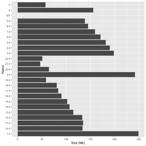
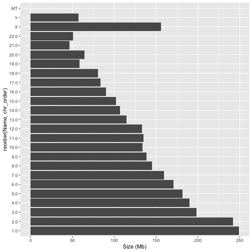
Notice how ggplot reorders the chromosomes in an unnatural way. This is because the Name field is of type character and ggplot will impose alphabetical ordering on it.
A good way to address this issue is to create an extra column that encodes the order with a numerical variable. For the chromosome table above this is easy because the chromosomes are already provided in the correct order. We can therefore add a column with the row number as follows;
readxl::read_excel("data/Chromosomes.xlsx", na = "-") |>
  mutate(chr_order = row_number())
## # A tibble: 25 × 13
##    Type  Name  RefSeq    INSDC `Size (Mb)` `GC%` Protein  rRNA  tRNA `Other RNA`
##    <chr> <chr> <chr>     <chr>       <dbl> <dbl>   <dbl> <dbl> <dbl>       <dbl>
##  1 Chr   1.0   NC_00000… CM00…        249.  42.3   11378    17    90        4605
##  2 Chr   2.0   NC_00000… CM00…        242.  40.3    8495    NA     7        3850
##  3 Chr   3.0   NC_00000… CM00…        198.  39.7    7559    NA     4        2849
##  4 Chr   4.0   NC_00000… CM00…        190.  38.3    4780    NA     1        2258
##  5 Chr   5.0   NC_00000… CM00…        182.  39.5    4828    NA    17        2280
##  6 Chr   6.0   NC_00000… CM00…        171.  39.6    5745    NA   138        2583
##  7 Chr   7.0   NC_00000… CM00…        159.  40.7    5357    NA    22        2480
##  8 Chr   8.0   NC_00000… CM00…        145.  40.2    4156    NA     4        2025
##  9 Chr   9.0   NC_00000… CM00…        138.  42.3    4709    NA     3        2289
## 10 Chr   10.0  NC_00001… CM00…        134.  41.6    5531    NA     3        2234
## # ℹ 15 more rows
## # ℹ 3 more variables: Gene <dbl>, Pseudogene <dbl>, chr_order <int>
We can now adjust our plotting code, making use of the function reorder to tell ggplot a column to use for the ordering
readxl::read_excel("data/Chromosomes.xlsx", na = "-") |>
  mutate(chr_order = row_number()) |>
  ggplot(aes(x=`Size (Mb)`,y=reorder(Name,chr_order))) +
  geom_col()
STOP Answer Questions 4-8 in the exercises
Regular Expressions
Earlier in this guide we extracted human gene entries into a file called human_genes.gff. In doing this we used grep, which is a command-line tool that searches for patterns in text. The name grep comes from g/re/p, a command in an old text editor that means globally search for a regular expression and print the matching lines. grep uses a specialised syntax called regular expressions to specify the patterns for searching. Our first encounter with regular expressions was the expression
^#
This uses the special character ^ to indicate that the match should start from the beginning of the text. Then the # indicates a character to match.
Aside from ^, there are many other special characters used in regular expressions. Some of the most common are;
| Operator | Description |
|---|---|
^ |
Match the start of the text |
$ |
Match the end of the text |
. |
Match any character |
[0-9] |
Match a numeric digit between 0 and 9 |
\w |
Match a word character |
* |
Match the preceding character (or group of characters in square brackets) zero or more times |
+ |
Match the preceding character (or group of characters in square brackets) one or more times |
[^<char>] |
Where <char> stands for a group of characters. Match any character except those in <char> |
When you write a regular expression in R it goes inside a string, and a backslash in an R string must itself be escaped. This means that \w is written as "\\w" in R code.
The full syntax of regular expressions is fairly complex, and is made extra difficult by the fact that different regex engines sometimes work differently. Don’t let this put you off though. If you learn just a few basic features of regular expressions you can accomplish a great deal.
As an example for working with regular expressions let’s take the first 10 entries in the human_genes.gff file that we created earlier. We can do this in R as follows;
gff_cols <- c("seqid","source","type","start","end","score","strand","phase","attributes")
gff10 <- read_tsv("cache/human_genes.gff",col_names = gff_cols,comment = "#", n_max = 10)
Inspect the 9th column of this dataset (called attributes). It has entries that look like this;
"ID=gene-MIR6859-1;Dbxref=GeneID:102466751,HGNC:HGNC:50039,miRBase:MI0022705;Name=MIR6859-1;description=microRNA 6859-1;gbkey=Gene;gene=MIR6859-1;gene_biotype=miRNA;gene_synonym=hsa-mir-6859-1"
Notice how all the entries in the attributes column are structured into key-value pairs separated by a semicolon “;”. For example;
ID=gene-MIR6859-1
Dbxref=GeneID:102466751,HGNC:HGNC:50039
Now let’s try some simple regular expression matching on this field. If we want to filter for rows that match a regex we can use the str_detect() function (from the stringr package) in conjunction with filter() from dplyr. For example, this code will extract only rows corresponding to genes that encode a particular type of transcript called a microRNA (miRNA);
gff10 |> filter(str_detect(attributes,"gene_biotype=miRNA"))
## # A tibble: 3 × 9
##   seqid        source     type   start    end score strand phase attributes
##   <chr>        <chr>      <chr>  <dbl>  <dbl> <chr> <chr>  <chr> <chr>
## 1 NC_000001.11 BestRefSeq gene   17369  17436 .     -      .     ID=gene-MIR685…
## 2 NC_000001.11 BestRefSeq gene   30366  30503 .     +      .     ID=gene-MIR130…
## 3 NC_000001.11 BestRefSeq gene  187891 187958 .     -      .     ID=gene-MIR685…
MicroRNAs are a particularly interesting type of gene product. They don’t encode proteins, but are involved in regulating expression of other genes. If we want to extract the entries for protein coding genes we could use;
gff10 |> filter(str_detect(attributes,"gene_biotype=protein_coding"))
## # A tibble: 2 × 9
##   seqid        source     type   start    end score strand phase attributes
##   <chr>        <chr>      <chr>  <dbl>  <dbl> <chr> <chr>  <chr> <chr>
## 1 NC_000001.11 BestRefSeq gene   65419  71585 .     +      .     ID=gene-OR4F5;…
## 2 NC_000001.11 Gnomon     gene  350706 476822 .     -      .     ID=gene-LOC112…
Now what if our goal was not just to filter rows, but to extract the value of gene_biotype in every row. This can be accomplished using another aspect of regular expressions, called a capture group. If we want to capture a portion of text that matches a pattern we can simply enclose the pattern in parentheses (<pattern>). To actually perform the extraction we use the function extract() from the tidyr package. Its arguments are the column to extract from (attributes), the name of the new column to create ("biotype") and the regular expression. Here is an example;
gff10 |> extract(attributes, "biotype","gene_biotype=([^;]*)")
## # A tibble: 10 × 9
##    seqid        source     type   start    end score strand phase biotype
##    <chr>        <chr>      <chr>  <dbl>  <dbl> <chr> <chr>  <chr> <chr>
##  1 NC_000001.11 BestRefSeq gene   17369  17436 .     -      .     miRNA
##  2 NC_000001.11 Gnomon     gene   29926  31295 .     +      .     lncRNA
##  3 NC_000001.11 BestRefSeq gene   30366  30503 .     +      .     miRNA
##  4 NC_000001.11 BestRefSeq gene   34611  36081 .     -      .     lncRNA
##  5 NC_000001.11 BestRefSeq gene   65419  71585 .     +      .     protein_coding
##  6 NC_000001.11 Gnomon     gene   89006 267354 .     -      .     lncRNA
##  7 NC_000001.11 BestRefSeq gene  134773 140566 .     -      .     lncRNA
##  8 NC_000001.11 BestRefSeq gene  187891 187958 .     -      .     miRNA
##  9 NC_000001.11 Gnomon     gene  200442 203983 .     +      .     lncRNA
## 10 NC_000001.11 Gnomon     gene  350706 476822 .     -      .     protein_coding
There is a fair bit going on in the regular expression here. Let’s start with the part inside the capture group, which is [^;]*. This part in square brackets matches any character except for a semicolon. This is useful because the semicolon delimits each entry in the attributes string. The * after the square brackets indicates that any number of characters should be matched (except for a ;). The text that comes before the capture group effectively anchors the match by searching for text that matches gene_biotype=. This ensures that the capture group will start after this text and continue until the first semicolon.
STOP Answer Questions 9-10 in the exercises