BC3203
Goal
Learn the fundamentals of the R language. A strong grounding in these concepts is essential in order to understand more advanced topics in R that will be encountered in later tutorials.
Setup
Setup RStudio to work with a clone of this repository and make sure you understand how to submit your edits so that they can be graded. This is all explained in the guide to tutorial 1.
How to complete this tutorial
Start by reading this document (you are in the right place). Do the exercises when instructed.
The assessable component is contained within the file exercises.Rmd. Open this file by clicking on it in RStudio. This is where you should enter answers to your questions. Your mark for this tutorial will be obtained from your answers to questions in this file.
You might also want to create a new RMarkdown document where you can practise commands. Give it a name that makes it clear that this is not your final answers (eg exploration.Rmd or practise.Rmd). Running practise code is a very important part of the learning process. You should feel free to add practise code to this file or to simply run it in a Terminal window. Important This file is for practising only. We will ignore everything in this file when marking assignments.
Running R tests
Since this tutorial is based around R it uses a slightly different testing framework to the one used for bash tutorials. Most things work the same but there are a few differences;
- Many questions will ask you to write your code in the form of a function. When you see questions of this type you must give your function the exact name specified in the question.
- Note that many questions will run multiple tests on your answer. Your answer will only be considered correct if all the tests pass.
- The R testing framework gives much better feedback on incorrect tests. If your test is failing try reading the test output. It might be useful.
In addition, in order for R tests to work you must first install the following R packages;
testthattidyverse
Guide
Fundamentals of the R language
Variables
Assignment and retrieval of variables in R works much like BASH but with slightly different syntax.
The code below shows two different ways to assign a value to the variable x. Both are syntactically valid but according to the style guide you should use <- rather than = for assignment.
x <- 1
message("x is ",x)
x = 2
message("x is ",x)
Printing to the console
Note that in the example above we used the message function. The is a bit like the echo command in BASH. You can use it to print some text as well as the value of a variable to the console.
There are several other ways to print a variable to the console. Try these out;
greeting <- "Hello"
cat("The greeting is ",greeting,"\n")
message("The greeting is ",greeting)
print(greeting)
greeting
R as a calculator
The table below lists some of the standard operators for performing calculations in R.
| Symbol | Operation | Example |
|---|---|---|
+ |
Add | 1 + 2 |
- |
Subtract | 1 - 2 |
* |
Multiply | 2*2 |
/ |
Divide | 1/2 |
^ |
Take to power | 2^3 |
%% |
Modulus (remainder) | 2 %% 3 or 3 %% 3 |
Try pasting the examples into the console and make sure you understand the result.
If you are new to programming, the modulus operator (%%) might be new. Play around with various values to get a feel for what it does.
Functions
In the BASH tutorial we mentioned that variables were a form of abstraction. A variable allows us to represent data in an abstract way, which enables useful things like loops.
Functions are another form of abstraction. This time instead of capturing data, a function captures a set of instructions that allow us to transform some input data into an output.
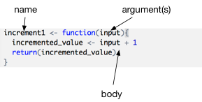
The following code creates a function that adds 1 to its input
increment1 <- function(input){
  incremented_value <- input + 1
  return(incremented_value)
}
Let’s break this code apart to see what the various components are. Firstly remember that this code is just the definition of the function. It doesn’t actually do any calculations yet (that comes later). It creates a new function object with the name increment1. The argument of the function in this case is called input it is a placeholder name for data that will be given to the function when it runs. Finally the body of the function contains the actual calculations. The body contains two lines. The first line takes the input value, adds 1 to it and assigns that to a new variable called incremented_value. The last line of the body declares that the value returned to the user of the function should be incremented_value. In R the return statement is actually optional. If there is no return statement the value of the last evaluated expression is automatically returned.
The code below will call the function with the value 3 used as input. When you run this code you will be using the function that you defined above to actually do something.
increment1(3)
- Try changing the function body to add 2 to the argument instead of 1 (call the function to test)
- Try changing the name of the function from increment1 to increment2. Observe that you need to change the way you call the function.
A note about return values from functions
The definition of the function incremement1 above uses an R built-in function called return to end the function and indicate the value that should be given back (returned) to the caller of the function. Another way of thinking of return is like a function’s output. The return statement determines the output of the function.
It turns out that the return statement is not usually needed. By default R will always return the result of evaluating the last expression in the function. So our increment1 function above could be written much more succinctly as;
increment1 <- function(input){
  input + 1
}
Stop: Answer questions 1-3 in the exercises before proceeding further
Logical Values and If Statements
A situation that often arises in programming is the need to take different actions depending on a condition. In order to accomplish this we need to introduce two new concepts. The first concept is logical values. A logical value can be either TRUE or FALSE. The following code produces a logical value
2 == 1 + 1
In this expression the double equals symbol, == is being used to test whether the expression on the left (2) is equal to the expression on the right (1 + 1). The result of this test is a logical value. In this case TRUE is returned because the expression is true.
The following operators all produce logical values
| Operator | Name | Example evaluating to TRUE |
|---|---|---|
< |
Less than | 1 < 2 |
> |
Greater than | 2 > 1 |
<= |
Less than or equal to | 1 <= 1 |
>= |
Greater than or equal to | 1 >= 1 |
!= |
Not equal to | "A" != "B" |
== |
Equal | "A" == "A" |
%in% |
Test for in group membership | "B" %in% c("A","B","C") |
Try out a few of these examples in the console. All of the examples evaluate to TRUE. See if you can change them to evaluate to FALSE.
Now that we know how to write tests to produce logical values we can potentially write code to perform different actions depending on whether a condition is true or false. This is accomplished with if statements.
An if statement in R has the following syntax
if (test_expression) {
statement
}
The idea here is that the code represented by statement will only be run if test_expression evaluates to TRUE. Here is an example;
x="A"
if ( x == "B" ){
  cat("x is equal to B")
}
if ( x == "A" ){
  cat("x is equal to A")
}
Often an if statement is paired with an else so that we can define one action to take if an expression is true and a different action to take if the expression is false
x="A"
if ( x == "B" ){
  cat("x is equal to B")
} else {
  cat("x is something else")
}
A note about cat and return
Look carefully at the two functions below;
display_hello <- function(){
  cat("hello")
}

return_hello <- function(){
  # Or equivalently
  #return("hello")
  "hello"
}
Try running these two functions? Can you spot the difference in their output?
display_hello()
## hello
return_hello()
## [1] "hello"
Now try assigning the result of each of these functions to a variable
dh <- display_hello()
## hello
rh <- return_hello()
Inspect the value of dh and rh. Notice how when display_hello() is run it always displays “hello” but the value that gets returned by this function is actually NULL and this is what will be stored in the variable dh. This is because cat doesn’t actually return anything. The effect of running cat it to produce a “side effect” of printing text to the screen.
On the other hand return_hello() actually returns the text “hello”. You can see this by printing the rh variable.
Understanding these concepts can be a little tricky at first. The main thing to remember is that if you are asked to “return” a value you should almost never use cat to do so.
Stop: Answer questions 4-5 before continuing
Vectors
Vectors are collections of values. Usually the values will one be one of the R fundamental data types
| Type | Example |
|---|---|
| character | “b” , “atgcg” |
| numeric | 3, 2.3 |
| integer | 1L |
| logical | TRUE, FALSE |
| complex | 2+2i |
In bioinformatics we regularly work with the first five of these types
A vector can be constructed using the c() function. Here are some examples;
greeting <- c("H","e","l","l","o")
powers_of_two <- c(2,4,8,16)
Vectors cannot contain data of different fundamental types so if you try to make a vector with different types R will try to automatically convert them. Often this means converting to character.
important_question <- c("Episode ",4," is the best star wars movie ",TRUE, "or", "FALSE")
important_question
The class() function can be used to find out the type of an object if it is not known. Errors arising due to data type conversions are probably the most common source of frustration for new R programmers. Use the class() function to make sure your data is the type that you expect.
class(important_question)
Here’s an example to illustrate why automatic class conversion might trip you up.
Here we have a vector of type numeric. It might be a set of data that you want to do calculations on. For example calculate the mean()
v_doub <- c(1.2,1.3,1.4,1.5)
mean(v_doub)
At some point you try to add an object of type character to the vector. When we try to perform the calculation we get an error
v_doub[5] <- "1.6"
mean(v_doub)
The c() function can also be used to join vectors together. Technically c() always joins vectors together because as it happens all of Rs fundamental types are always vectors. Individual values like 1, "a" etc are just vectors of length 1.
c(greeting,c(" "),c("W","o","rl","d"))
You can find out the length of a vector with the length() command
x <- c("a","b","c")
length(x)
Vectorised operations
Operations that work for individual values also work for vectors. For example;
v_numeric <- c(0.5,1.1,-1,2)
v_logic <- v_numeric > 0
v_squared <- v_numeric*v_numeric
v_by2 <- v_numeric*2
Try running each of the four examples above by pasting into R. Inspect the resulting value in each case.
Retrieving values within vectors
The items within a vector can be retrieved by their index using square brackets [ ]. The first item has index 1, the second has index 2 and so on.
greeting <- c("H","e","l","l","o")
Access a single item
greeting[3]
Several items can be accessed at once using another vector of integer indices
greeting[c(1,2,3)]
You can also specify items not to retrieve using -
greeting[-1]
greeting[-c(1,5)]
This principle also extends to using logical vectors as indexes. A value of TRUE means that the item should be retrieved whereas a FALSE means that it will not.
For example;
dice_rolls <- round(runif(10,1,6))
dice_rolls

# Retrieve all rolls > 3
dice_rolls[dice_rolls>3]
If we try to retrieve an index outside the bounds of a vector, we get a special symbol, NA which stands for not available. Missing values in R are generally represented by NA.
length(dice_rolls)
dice_rolls[11]
Named Vectors
Items within a vector can also be named. For example;
numbers <- c("one" = 1, "two" = 2, "three" = 3, "four" = 4)
numbers
Items in a named vector can be accessed by name, (as well as by index)
numbers[c("two","three")]
numbers[c(2,3)]
A named vector can be used like a dictionary to lookup from a table of values. One example where this might be useful is when obtaining the complement of a DNA base.
# This constructs the dictionary
bases <- c("A","T","C","G")
comps <- c("T","A","G","C")
names(comps) <- bases

# These show usage of the dictionary to lookup different complementary bases
comps["A"]
comps["T"]

# Or we could lookup the complement from a base stored in a variable
b <- "C"
comps[b]
Stop: Answer question 6 in the exercises before going further
Generating vector indexes
Retrieving values from large vectors can be done in a variety of ways with R. One of the most powerful methods is to use the seq() function.
Look at the R help page for seq to see what it does.
Try a few examples
seq(1,10)
seq(10, 1, by = -2)
Another shorthand method is to use the : operator.
2:5
7:2
Stop: Answer question 7-12 in the exercises before going further
Loops
Like all programming languages R provides mechanisms for performing actions repeatedly. One way is to use a loop. There are several ways to write loops in R but for now we will stick with for loops and will use syntax that is fairly similar to the way for loops work in BASH. The syntax for a for loop in R is;
for (variable in vector) {
  expression
}
For example;
x2 <- c()
for (x in 1:10) {
  x2 <- c(x2,x*2)
}
x2
This loop constructs a new vector x2 which is each element of the vector 1:10 multiplied by 2. You probably already can see that this isn’t the easiest way to accomplish this. Instead of a loop this could have been done using vectorised multiplication like this
x <- 1:10
x2 <- x*2
x2
This is not only more succinct, it is also much faster since the vectorised * operator is highly optimised. As a general rule any time you can use a vectorised operation instead of a for loop you should do so. Loops in R are sometimes necessary but should be avoided if possible.
Stop: Answer questions 13-14 in the exercises before going further
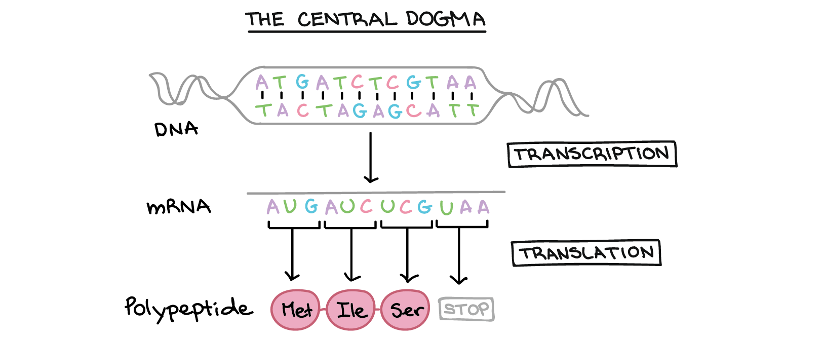
Translating DNA to Protein
In this section you will write R functions to translate a sequence of DNA nucleotides A,G,C and T into a protein sequence. The code you write will computationally reproduce the process by which proteins are made from genes. This involves transcription of a DNA sequence into RNA followed by translation into protein.
Data Resources
This tutorial comes with a tabular file that provides the standard genetic code. The genetic code consists of a set of triplets of DNA (called codons) along with the amino acid which that codon is translated to.
Load the genetic code as follows;
library(tidyverse)
genetic_code <- read_tsv("data/genetic_code.tsv")
This code requires the tidyverse package to be installed.
Note that there are 64 rows in this table corresponding to the 64 possible 3 letter combinations of A,G,C and T. The first two columns of the table are self-explanatory. They represent the three letter DNA codon and the corresponding amino acid respectively. Ignore the Start column for now. It denotes codons that can act as start sites for translation. If a codon is a start site it always codes for Methionine M even if it might code for an alternative amino acid when it is not the starting codon. We will ignore this complexity for now.
Values in the AA column consist of the 20 possible amino acids as well as a * symbol which denotes a stop codon. If a stop codon is encountered, translation will stop at that point. Translation generally starts at a start codon (Methionine) and ends at a stop.
For the purposes of this tutorial we will work with a relatively short DNA sequence which codes for the protein CAMP_HUMAN. Using a short sequence like this as an example will make it easier to write and debug your code.
The code below creates a single long DNA string with the sequence for CAMP_HUMAN. In case you are wondering the use of gsub() is just to remove whitespace (ie spaces, linebreaks) in the string.
dna <- gsub("\\s+","",
"ATGGGGACCATGAAGACCCAAAGGGATGGCCACTCCCTGGGGCGGTGGTCACTG
GTGCTCCTGCTGCTGGGCCTGGTGATGCCTCTGGCCATCATTGCCCAGGTCCTCA
GCTACAAGGAAGCTGTGCTTCGTGCTATAGATGGCATCAACCAGCGGTCCTCGGA
TGCTAACCTCTACCGCCTCCTGGACCTGGACCCCAGGCCCACGATGGATGGGGAC
CCAGACACGCCAAAGCCTGTGAGCTTCACAGTGAAGGAGACAGTGTGCCCCAGGA
CGACACAGCAGTCACCAGAGGATTGTGACTTCAAGAAGGACGGGCTGGTGAAGCG
GTGTATGGGGACAGTGACCCTCAACCAGGCCAGGGGCTCCTTTGACATCAGTTGT
GATAAGGATAACAAGAGATTTGCCCTGCTGGGTGATTTCTTCCGGAAATCTAAAG
AGAAGATTGGCAAAGAGTTTAAAAGAATTGTCCAGAGAATCAAGGATTTTTTGCG
GAATCTTGTACCCAGGACAGAGTCCTAG")
Constructing codons from a dna string
The first step in translating DNA to protein involves identifying the codons (DNA triplets) within a long DNA sequence.
In order to accomplish this we can use the substring() function to split our dna sequence into pieces. Look at the R help for the substring() function like this;
help(substring)
You should see that substring() is designed to extract parts (substrings) of a character vector (a string). It takes 3 arguments; The first argument is the original string we are working with (ie dna from above). The second argument is the starting point for the substring to extract and the third argument is the end point of the substring to extract.
For example we could get the first codon in our dna string like this.
substring(dna,1,3)
This becomes much more useful when you discover that substring takes vectors as arguments. This allows extraction of more than one substring at once. For example this will extract the first two codons in the dna string.
start_positions <- c(1,4)
end_positions <- start_positions+2
substring(dna,start_positions,end_positions)
Now recall from previous exercises that the seq() function can be used to generate sequences of numbers. The trick to answering question 15 will be in combining the seq() and substring() functions in the correct way. Also note that to get the length of a string you will need to use the nchar() function.
Stop: Answer question 15 in the exercises.
Translating DNA to protein
Good programming often comes down to getting data into the right format. In order to translate DNA to proteins we need a way to map codons (as generated with the dna_to_codons function you wrote in the previous question) into amino acids. This information is encoded in the genetic_code table but is not in a convenient format.
Remember that with a named vector it is possible to lookup elements of the vector based on their names. So for example;
codons_to_aa <- c("TTT" = "F","TTC" = "F", "TTA" = "L")
codons_to_aa[c("TTA","TTA","TTC","TTT")]
We can convert the columns of genetic_code directly into a named vector using the function names() as follows;
codons_to_aa <- genetic_code$AA
names(codons_to_aa) <- genetic_code$Codon
Stop: Answer question 16 in the exercises
Translation in forward reading frames
Up the this point we have assumed that our DNA sequence should be translated starting from the first base. What if we started from the second base? or the third? If we did this we would obtain a completely different protein sequence.
In practise it is often difficult to determine the exact starting point of translation for a DNA sequence. It is common to scan unknown sequences of DNA by translating in all possible reading frames.
Stop: Answer question 17 in the exercises
Translation in reverse frames
DNA is double stranded and transcription can occur on either strand. This means that a DNA sequence could potentially encode a protein sequence in six possible reading frames. These correspond to three possible forward frames (see above) as well as three additional frames that arise by translating the reverse complement of the sequence.
Stop: Answer question 18 in the exercises
Recursion (Optional Challenge)
Recursion
A recursive function is a function that calls itself within its body. This can be an extremely powerful technique for traversing certain types of biological data (phylogenetic trees for example).
Writing recursive functions is not hard but there is one important trick. You must ensure that the recursion does not continue indefinitely.
For example the code below would run forever. (Actually it produces an error because it exceeds the maximum stack size)
infinite_recursion <- function(x){
  infinite_recursion(x)
}
infinite_recursion()
A more sensible example would be the following
integer_sequence <- function(start,end){
  if ( start >= end ){
    return(start)
  }
  c(start,integer_sequence(start+1,end))
}

integer_sequence(1,10)
Note that in this example we used the return function to force an early return from the function body. By default R will start at the top of the function body and evaluate all code from top to bottom with the final result automatically being returned as output. In the example above we want the recursion to stop if (start >= end) so we use return to prevent the final line of code in the body from being run during the last stage of recursion.
Also note the use of the c function to concatenate vectors which we will cover in more detail below.
Useful information for questions 19 and 20
The factorial of a number n is defined as;
\[n! = n(n-1)(n-2)...(2)(1)\]The Fibonacci sequence is defined by the following recurrence relation;
\[F_n = F_{n-1} + F_{n-2}\]This means every number after the first two is the sum of the two preceding ones. You should seed your sequence with starting values as $F_{n-1}=1$, $F_{n-2}=0$
Stop: Answer questions 19 and 20 in the exercises