BC3203
Major Assignment 1 : Metagenomics
Goal
This goal of this guide is to walk you through a complete analysis of 16S metagenomic data using QIIME. It is designed to prepare you for completing the assessable component. As you work through you should try to understand what is happening at each step. The more you can learn from this guide the easier it will be for you to solve problems in the assessable part of the assignment.
Setup
Start by visiting the assignment invite link, https://classroom.github.com/a/PWO1Bp9j and clicking accept. After you accept the assignment your own personal copy will be created on github. Create a new project in RStudio by cloning the assignment from github. This is the same procedure that is used for all the coding assignments and tutorials.
Keeping track of what you are doing
As you run commands you should keep a clear record of what you have done. I strongly recommend that you create a new RMarkdown document for this purpose. This document is for your own record keeping and will not be assessed. Nevertheless, I recommend that you add this document to git and commit/push it to github regularly. This will ensure that if anything happens to our server, or if you accidentally delete your notes you will have a “backup” on github.
Since you will be committing changes to github regularly you should try to write meaningful commit messages. If you ever need to look back at a previous version of a command these will help. I recommend messages like “completed deblur step”, or “finished part 1 of the report”.
Your github commit log will form a component of your assessment. Assignments that make a single large commit at the end will be flagged for further scrutiny since this is a potential sign of plagiarism.
Completing the Assessment
After completing the guide (see below) you should open the file report.Rmd and edit it as instructed. This file will contain all your work for assessment. You will need to delete the instructional text in your own copy of report.Rmd. If you want to see the original instructions at any point you can see them at this link.
Submitting your assignment
See LearnJCU for the due date for this assignment.
You should submit your assignment as follows;
-
Make sure you have pushed your latest changes to github by the due date.
-
Use the
knitfunction in RStudio to compile your assessable report into pdf format. Download the resulting pdf and submit this through LearnJCU SafeAssign.
Please note that you MUST submit your assignment in pdf format. Getting the “knit to pdf” function to work is part of the assessment. If you leave this until right at the end it will often fail and be difficult to debug. I recommend that;
- Knit to pdf before you make any edits to
report.Rmd. This serves as a test to make sure the knitting process is working - Knit to pdf whenever you make any substantial change to
report.Rmd. If it doesn’t work you will know that something about the most recent edit is at fault. Stop right there and debug before you move on.
Marking Criteria
This assignment is assessed according to its presentation and content. Marks will be allocated according to standards documented in the subject outline. Report sections will be assessed on the quality of presentation (language, spelling, logical flow and structure of text / figures etc), clarity of insight, use of appropriate terminology. As described in the report template you must demonstrate a good technical understanding of the steps included in your analysis. This will comprise a large proportion of the marks for sections 1 and 2.
A breakdown of marks for different components of the assignment is as follows;
| Criterion | Guidelines | Marks |
|---|---|---|
| Git commit log | Meaningful messages, commits at sensible intervals (not all in one commit at the end). | 5% |
| Overall presentation | Appropriate use of RMarkdown to generate a cleanly formatted report | 15% |
| Report Section 1 | As per subject outline content and presentation guidelines | 40% |
| Report Section 2 | As per subject outline content and presentation guidelines | 40% |
Guide
This guide is a slightly elaborated version of the official qiime moving pictures tutorial available on the qiime website.
How to complete this guide
There are no questions or directly assessable items in this guide but completing it is a crucial learning experience that will prepare you for the assessable components. Be sure that you;
-
Complete the entire guide from top to bottom
-
Run each of the commands in the guide. Most of the time this will involve copying and pasting commands from the guide into your terminal window.
-
It is highly recommended that as you keep notes on commands you are running (see above section on taking notes). For example you could create a file called
moving_pictures.Rmd. Cut and paste every command that you run into that file. Keep them in the correct sequence and take notes on the commands as you go. This is not assessable but is for your own reference. -
Take a minute to think about the commands you are running. Specifically you should;
- Look at the output of commands. You may not understand everything but you should have a general idea of what each command is designed to accomplish. Try to connect what you are doing with concepts learned in theory lectures.
- Check that your commands worked. Look for appropriate output files generated by commands. Read errors and warnings and make sure they are not fatal to the analysis.
Advice on running commands
Most of the commands you will be asked to run in this guide are bash commands. The best way to run them is to cut-paste (or type) them into a terminal window.
If you use an RMarkdown document to take notes you can also create bash code chunks within that document. Please take a look at this short video for my recommendations on how to write these code chunks.
Step 1 : Download and inspect raw data
The starting point for most metagenomics analyses will be a (potentially very large) set of fastq files as well as a tabular file describing each of the samples. The tabular file contains metadata that links the sequencing read data (in fastq files) to the experiment.
Both the sequencing reads and metadata should be considered read-only data. They form the starting point for our analysis and should never be modified. They are also fairly large so they should not be committed to our git repository.
In order to keep things organised we download our starting data to it’s own directory called raw_data. Your git repository is setup to ignore everything inside this folder so it will be safe from being committed to git.
Download the metadata directly to the raw_data folder using the following command;
wget -O "raw_data/sample-metadata.tsv" "https://data.qiime2.org/2023.5/tutorials/moving-pictures/sample_metadata.tsv"
Download reads and corresponding barcodes using the following commands;
mkdir -p raw_data/emp-single-end-sequences

wget -O "raw_data/emp-single-end-sequences/barcodes.fastq.gz" "https://data.qiime2.org/2023.5/tutorials/moving-pictures/emp-single-end-sequences/barcodes.fastq.gz"

wget -O "raw_data/emp-single-end-sequences/sequences.fastq.gz" "https://data.qiime2.org/2023.5/tutorials/moving-pictures/emp-single-end-sequences/sequences.fastq.gz"
Note: We store reads and barcodes in a subfolder of raw_data called emp-single-end-sequences. This is to support QIIME import steps that come later.
What are the barcodes?
Modern sequencers are capable of sequencing a very large number of DNA molecules in a single run. This number of reads is sufficient to support the analysis of many samples simultaneously so it is now very common to run multiple samples on a single run. Barcodes are added to each sample so that reads for each sample can then be separated based on barcode after sequencing. This is an example of multiplexing.
Securing raw data
Inspect the unix permissions on the data we downloaded
ls -l -R raw_data/
## total 16
## -rw-r--r--@ 1 sci-irc  staff   215 May 11  2018 README.md
## drwxr-xr-x@ 4 sci-irc  staff   128 Mar  4 06:45 emp-single-end-sequences
## -rw-r--r--@ 1 sci-irc  staff  2094 Jul 13  2021 sample-metadata.tsv
##
## raw_data//emp-single-end-sequences:
## total 56816
## -rw-r--r--@ 1 sci-irc  staff   3783785 Mar  2  2021 barcodes.fastq.gz
## -rw-r--r--@ 1 sci-irc  staff  25303756 Mar  2  2021 sequences.fastq.gz
The files are readable by all users which is fine, but the owner of the files is able to modify them ( w - write ). To make sure the files won’t be modified we can remove this permission as follows;
chmod u-w raw_data/emp-single-end-sequences/*.gz
chmod u-w raw_data/*.tsv
After doing this inspect permissions again to make sure it worked.
Inspecting raw data
The following command demonstrates how to inspect the first few lines of a gzipped fastq file without unzipping the entire file.
gunzip -c raw_data/emp-single-end-sequences/barcodes.fastq.gz | head
This is fastq formatted data which means that each barcode is represented by 4 lines. In order to count the number of barcodes we could count the number of lines and then divide by 4. This is easily done using awkas follows;
gunzip -c raw_data/emp-single-end-sequences/barcodes.fastq.gz | awk 'END {print NR/4}'
awk is a simple language for text processing. It is very powerful and very useful to learn because it is built into every unix-like system. We will only briefly touch on awk in this course. Here is a quick explanation of the command above;
-
The command starts with
ENDas its pattern which tells awk to wait until it reaches the end of the file before running the program (the part between curly brackets{}). -
The awk program uses the keyword
printwhich prints the valueNR/4. -
NRstands for “Number of Records” where each record is a line. SoNR/4would be the total number of lines at the end of the file divided by 4.
Now run the code below to count the number of sequences in the sequences file
gunzip -c raw_data/emp-single-end-sequences/sequences.fastq.gz | awk 'END {print NR/4}'
Counting the number of entries in barcodes and sequences should have revealed that both files have the same number of sequences. This is because every sequence has a barcode.
The barcodes assign sequences to samples as the image below illustrates;
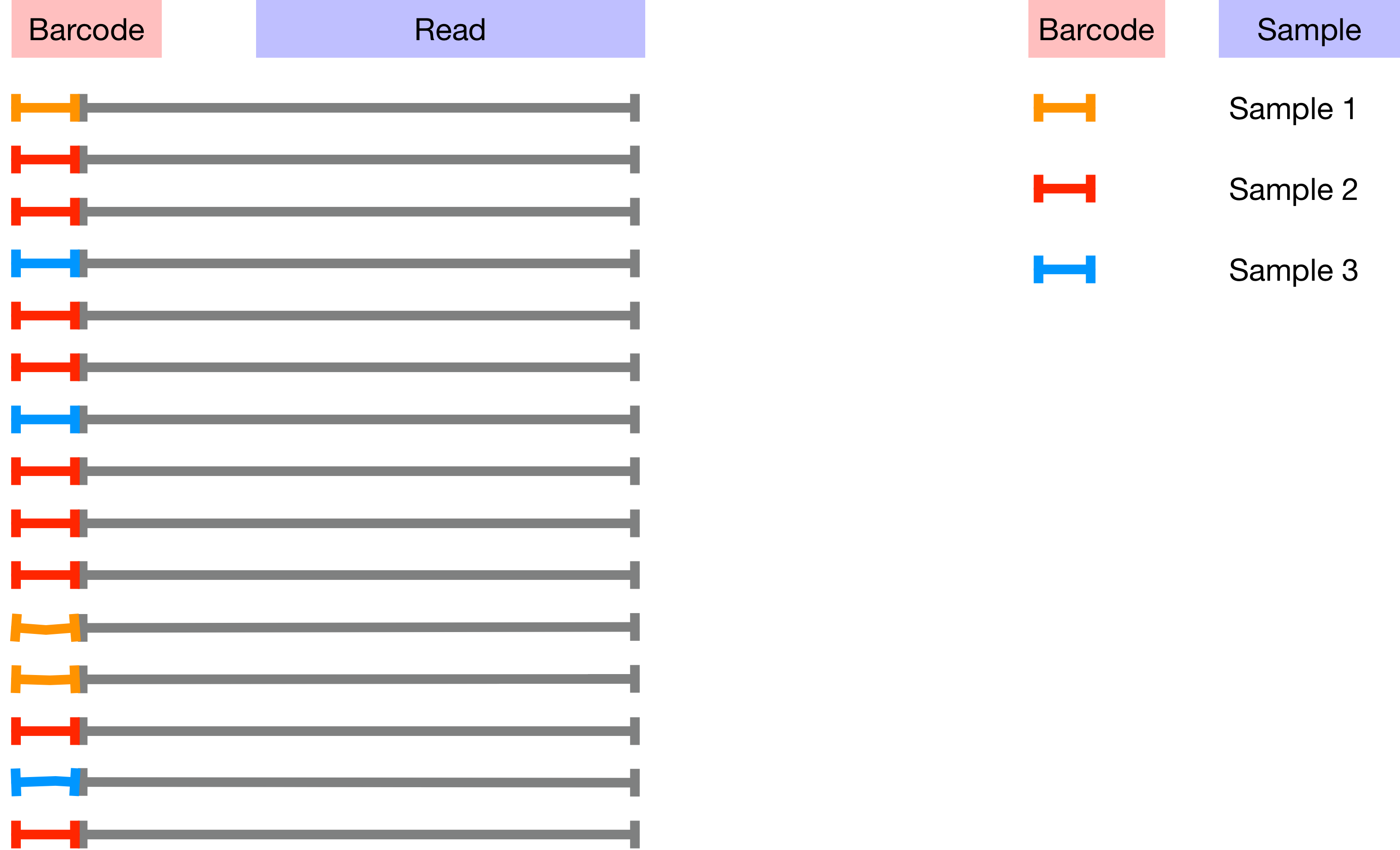
The mapping between samples and barcodes is given in sample-metadata.tsv. Use the code below to inspect sample-metadata.tsv and find the column corresponding to the Barcodes.
head -n 3 raw_data/sample-metadata.tsv
Barcodes are in the second column so you can use the command below to count the number of unique barcodes in sample-metadata.tsv. Note that every sequence in the sequences file is unique but many of the barcodes will occur multiple times. This is because (in theory) all of the sequences for each sample should have the same barcode.
cat raw_data/sample-metadata.tsv | grep -v '^#' | awk '{print $2}' | sort -u | wc -l
Don’t worry if you don’t fully understand how this command works. There are a few important things to note about it. Firstly take note of the pipes |. There are four pipes which separate five commands. Imagine the data starting on the left-most command and passing through the pipes. Each time it passes through a pipe it gets passed as input to the next command as follows;
cat raw_data/sample-metadata.tsvreads the data and sends it to the next commandgrep -v '^#'removes all lines that start with a#symbol- `awk ‘{print $2}’ prints the second column of each line
sort -usorts all lines alphabetically and then removes duplicateswc -lcounts the number of remaining lines.
Based on the number of unique barcodes in the sample-metadata how many unique barcodes would you expect to find in the barcodes.fastq.gz?
Run the code below to determine the actual number of unique barcodes present in the barcodes.fastq.gz.
gunzip -c raw_data/emp-single-end-sequences/barcodes.fastq.gz | awk 'NR % 4 ==2' | sort | uniq | wc -l
There are many more unique barcodes in barcodes.fastq.gz than in sample-metadata.tsv. Your first assessment task (see report.Rmd) requires you to investigate and resolve this discrepancy.
Import barcodes and sequences into a QIIME artifact
As a final step for this part of the assignment we will import the sequences and barcodes into a QIIME artifact.
To keep things neat and to avoid accidentally committing large files or temporary analysis files into github we store all qiime results (including artifacts and visualisations) in a separate folder called qiime
qiime tools import \
  --type EMPSingleEndSequences \
  --input-path raw_data/emp-single-end-sequences \
  --output-path   qiime/emp-single-end-sequences.qza
After running this command check to make sure it generated a valid output file at qiime/emp-single-sequences.qza. One way to do this is to inspect the file using the qiime peek function. If everything worked this should report that the artifact type is “EMPSingleEndSequences” and the data format is “EMPSingleEndDirFmt”.
qiime tools peek qiime/emp-single-end-sequences.qza
Step 2 : Demultiplex
Having downloaded our data and given it a brief check we will now perform demultiplexing on it. This process uses the barcode-to-sample assignments present in the sample-metadata file to separate the reads according to sample.
Run the code below to perform the demultiplexing using the emp-single demultiplexing engine in qiime. This process takes a while (around 1 minute) so be patient when waiting for it to run.
qiime demux emp-single \
  --i-seqs qiime/emp-single-end-sequences.qza \
  --m-barcodes-file raw_data/sample-metadata.tsv \
  --m-barcodes-column barcode-sequence \
  --o-per-sample-sequences qiime/demux.qza \
  --o-error-correction-details qiime/demux-details.qza
Summarise demultiplexed sequences
Up to now you will have seen that we used qiime to create so called artifacts. These artifacts are useful as steps in an analysis pipeline but they are not particularly useful without a tool to inspect and summarise them. Fortunately qiime provides such a tool, called summarize. The next bit of code uses summarize to create a visualization object.
qiime demux summarize \
  --i-data qiime/demux.qza \
  --o-visualization qiime/demux.qzv
Now examine the visualisation file you created above (ie demux.qzv) using the qiime viewer. The qiime viewer is a web application that allows you visualise any qiime2 created visualisation file. If you are working from RStudio on the cloud you will first need to download the file to your local computer
Once you have downloaded the file you should be able to drag and drop it onto the qiime viewer.
Use the interactive viewer to answer the following (not assessable) questions.
-
How many samples have more than 10000 sequences?
-
At what position in the read does the median quality score first drop below 30?
-
Given that quality scores are Phred scaled what is the probability of error for Q30?
-
What is the total number of demultiplexed sequences? How does this compare with the total number of raw sequences (prior to demultiplexing)? What might account for the difference?
Step 3 : Denoise
Microbial communities can be highly diverse which means that any given sample might contain thousands of different true 16S sequences corresponding to different species and/or strains of microbes. If it was possible to obtain error free sequencing data we would expect to obtain a single representative sequence for all microbes belonging to a particular strain because they should be (almost) genetically identical.
In this step we deal with the fact that sequencing is not error free. Even Illumina sequencing generates errors when reading each base. In addition to this, the fact that 16S sequencing is based on amplification of many similar sequences means that we are likely to have chimeric reads which must be flagged and removed.
Both base calling errors and chimeras result in an inflation of the number of unique sequences in our data compared with what was actually in the sample. In this step our aim is to find reads that would have originated from the same real sequence, group them together and represent them using a single “representative sequence”. There are many methods for doing this. We will use Deblur. In lectures we discuss two broad approaches to denoising;
- Error modelling, which is implemented in Deblur and dada2
- OTU Clustering which is implemented in UPARSE
The error modelling approach is now favoured over OTU clustering in almost all circumstances. We chose to use Deblur for this tutorial just because it is easy to run within qiime but the dada2 approach is similar in principle.
Filter sequences by base call quality
Although Deblur takes quality scores into account it is best to trim sequences first to remove the very worst data. The code below uses the qiime quality-filter tool to do this. It’s default is to trim sequences to avoid any base calls with quality scores less than 4 on a Phred scale.
qiime quality-filter q-score \
 --i-demux qiime/demux.qza \
 --o-filtered-sequences qiime/demux-filtered.qza \
 --o-filter-stats qiime/demux-filter-stats.qza
Now use another qiime command to produce a visualisation of the filtering statistics
qiime metadata tabulate \
  --m-input-file qiime/demux-filter-stats.qza \
  --o-visualization qiime/demux-filter-stats.qzv
Download the visualisation file demux-filter-stats.qzv to your computer and visualize it using the qiime2 viewer.
The visualisation is just a table showing some statistics on how many reads were removed as a result of filtering. Each row in the table shows stats for a sample.
Use the button Download metadata TSV file to download the table and then upload it back to your RStudio instance. Rename the file to demux-filter-stats.tsv and save it in the qiime folder.
Now run the bash command below. This will print the sample name and the proportion of retained reads (to input reads) for each sample.
cat qiime/demux-filter-stats.tsv | tail -n +3 | awk '{print $1, $3/$2}'
Now run this bash command to print the average proportion of retained reads across all samples.
cat qiime/demux-filter-stats.tsv | tail -n +3 | awk 'BEGIN{av=0}{av+= $3/$2}END{print av/NR}'
A particularly low proportion of retained reads compared with the average could indicate a problematic sample. Note that this is just one of many ways that you could identify potentially problematic samples. You should usually try to avoid throwing away samples, but if a sample gives results far outside other replicates (ie an outlier) then these quality metrics can be used to decide where the problem arose (ie in sequencing, or in sample prep) and whether to discard the sample.
Denoise sequences
Now run deblur to reduce sequences down to a set of unique sequences representing the different organisms present in the sample. This step will also trim bases from the quality filtered reads as well as remove chimaeras.
How to deal with long running commands
This command takes a long time to run (about 10 minutes). Long running commands like this pose special problems. In particular we would like to;
-
Allow the command to run in the background so that we can keep working
-
Allow the command to keep running even if we logout of the server
-
Avoid crashing the server by putting it under too much load
Unfortunately if you simply run a long running command using the run button on an RMarkdown document (like this) you won’t achieve any of the goals listed above.
There are lots of ways to deal with long-running commands. Here we will use a queuing system called slurm. Systems like slurm are normally used in large clusters or supercomputers and can prioritise large numbers of jobs across many compute nodes. The JCU High Performance Computer system (JCU HPC) uses a similar system called PBS. Here I have installed slurm on our single node to allow the whole class to run longer jobs without crashing the server.
To run a command as a slurm job requires a little extra effort. Instead of simply typing the command in the Terminal and hitting enter we need to wrap our command into a short “job script”. In this case I’ve already done this for you so you can see what a job script looks like. Open the file called 03_deblur_slurm.sh by clicking on it in the file browser. It should show code that looks like this;
#!/bin/bash
#SBATCH --time=60
#SBATCH --ntasks=1 --mem=1gb

echo "Starting deblur in $(pwd) at $(date)"

apptainer run -B /pvol/:/pvol /pvol/data/sif/qiime.sif qiime deblur denoise-16S \
  --i-demultiplexed-seqs qiime/demux-filtered.qza \
  --p-trim-length 120 \
  --o-representative-sequences qiime/rep-seqs-deblur.qza \
  --o-table qiime/table-deblur.qza \
  --p-sample-stats \
  --o-stats qiime/deblur-stats.qza

echo "Finished deblur in $(pwd) at $(date)"
The three lines at the top that start with # are special. Let’s walk through them
#!/bin/bash
This tells slurm that we want to run our commands in the bash shell. This is the command line interpreter we are using for all our command line exercises.
#SBATCH --time=60
#SBATCH --ntasks=1 --mem=1gb
These lines are special instructions to slurm to tell it what physical resources our job will need. We are telling it that the job should not take more than 60 minutes --time=60, that it will use just one CPU --ntasks=1 and no more than 1Gb of memory --mem=1gb. These are quite important because slurm will use this information to figure out how many jobs it can safely run at the same time. Our goal when writing a slurm script should be to ask for just enough resources and no more. The numbers provided here should work well for this task.
echo "Starting deblur in $(pwd) at $(date)"
Next we have an echo command which will let us see when the job started. When the job starts running it will produce an output file. We can look that that file and should expect to see this information in there.
shopt -s expand_aliases
alias qiime='apptainer run -B /pvol/:/pvol /pvol/data/sif/qiime.sif qiime'
These commands are a little tricky to explain. The first one is needed because bash doesn’t expand aliases in non-login shells (don’t worry if you don’t know what that means) and slurm scripts are running in non-login shells. We need to explicitly tell the script to expand aliases because qiime is actually an alias. You can see this by running the following command
type qiime
This is telling you that when you type the qiime command the shell will automatically expand it into a much longer complicated command. The long complicated command is needed because qiime is installed within a singularity container on our system. Again you don’t need to know what all this means but just that we need to restate this alias in the slurm script so that it will be available when our command runs.
qiime deblur denoise-16S \
  --i-demultiplexed-seqs qiime/demux-filtered.qza \
  --p-trim-length 120 \
  --o-representative-sequences qiime/rep-seqs-deblur.qza \
  --o-table qiime/table-deblur.qza \
  --p-sample-stats \
  --o-stats qiime/deblur-stats.qza
Finally we have some lines which are just a normal qiime command.
OK so now we are ready to run the command. We do this as follows;
sbatch 03_deblur_slurm.sh
If everything is working you should see output like this
Submitted batch job <number>
Now your job should actually be running behind the scenes. There are several things you can do to check on it. Firstly try the squeue command. This will show all the queued and running jobs within the system. It might look something like this

Important parts of this to pay attention to are
- the
USERcolumn. You should look for your login id to find your job - the
STcolumn. This tells you the status of your job.Rmeans it is running. - the
TIMEcolumn tells you how long your job has been running for. - the
JOBIDcolumn gives a number identifying the job
If there are a lot of jobs in the queue it might be tricky to find yours. You can restrict the list to show only your job by using the -u option like this (where jcXXX is your login ID)
squeue -u jcXXX
If you realise that you made a mistake you can cancel a job with scancel. First find the JOBID number and then enter it like this
scancel JOBID
Once your job starts running it will produce output. Look for a file called slurm-JOBID.out where JOBID is a number. Take a look in this file to see output from your job at any time
cat slurm-JOBID.out
The command should take around 5-10 minutes to run. When it is finished it will disappear from the list in squeue. You can also check the output file and you will know that the job is finished because you will see output something similar to this;
Starting deblur in /home/test2023/metagenomics-iracooke-1 at Thu 03 Aug 2023 09:07:38 UTC
Saved FeatureTable[Frequency] to: qiime/table-deblur.qza
Saved FeatureData[Sequence] to: qiime/rep-seqs-deblur.qza
Saved DeblurStats to: qiime/deblur-stats.qza
Finished deblur in /home/test2023/metagenomics-iracooke-1 at Thu 03 Aug 2023 09:12:54 UTC
Inspect denoised outputs
Three output files are produced by the denoising step. We inspect each of them using qiime’s visualisation tools and the command-line
Representative sequences: Are sequences that represent a collection of very similar reads in the raw data. In theory each representative sequence should represent a different taxonomically distinct organism in the sample. These are contained in an artifact called rep-seqs-deblur.qza
Create a visualisation for the representative sequences identified by deblur
qiime feature-table tabulate-seqs \
  --i-data qiime/rep-seqs-deblur.qza \
  --o-visualization qiime/rep-seqs.qzv
Open the rep-seqs.qzv in the qiime viewer. This viewer will show you a list of sequences each of which is 120 bases long. A few things are worth noting;
- How many representative sequences are there in total? Why is this much less than the total number of reads/sequences in the experiment?
- Each sequence represents a fragment of the 16S gene from a particular organism. One way you could identify the organism itself is by performing a BLAST search of the sequence against a large database of known sequences. This is very easy in the
qiimeviewer. Just click the sequence itself and it will take you to a BLAST results page. Try this for a few sequences and take a look at the names of organisms that come up. Later on in this tutorial we will perform taxonomic classification of these same sequences using a machine learning classifier, which is a faster, more accurate approach.
Feature table: This artifact (called table-deblur.qza) contains counts of the number of occurrences of each representative sequence in each sample.
Create a visualisation for the feature table using the code below.
qiime feature-table summarize \
  --i-table qiime/table-deblur.qza \
  --o-visualization qiime/table-deblur.qzv
Inspect the visualisation using the qiime viewer. You should see that each sample is just labelled according to its code (eg L5S222). Naturally it would be much better if we could visualise the data along with information about the sample (eg which body site, antibiotic treatment etc).
In order to improve the visualisation you will need to remake it. This time you will need to include information from the sample-metadata.tsv file in raw_data/sample-metadata.tsv. To figure out how to do this you should inspect the help for the feature-table summarize tool in qiime (see below). Look for an option that would allow you to incorporate sample metadata.
qiime feature-table summarize --help
Remake the visualisation and then explore it in your web browser to answer. From which body site does the sample with the highest depth come from? (Note that you can find this out in the “Interactive sample detail” view by sliding the “Sampling Depth” indicator to the right until only one sample remains. The body site for this sample is the answer.)
Step 4 : Construct a phylogenetic tree from representative sequences
The previous step used Deblur to reduce the dataset from millions of individual reads down to just a few hundred distinct sequences. Each of these sequences represents a different organism present in the samples. In this step we examine the phylogenetic relationships between them. This allows us to identify sequences that are from closely related organisms versus those from more distant taxa. This will allow phylogeny based diversity metrics to be calculated in subsequent steps.
Align sequences
First create a multiple sequence alignment of all the representative sequences. The goal of multiple sequence alignment is to identify sections of the sequences that are homologous and line these up so that they occupy the same positions in the alignment.
To perform an alignment we use the program mafft. We don’t actually run mafft directly but use the qiime plugin for mafft.
The code below is broken. Try running the code. Look at the error that is produced and then fix the code
qiime alignment mafft \
  --o-alignment qiime/aligned-rep-seqs.qza
Inspect the alignment
qiime doesn’t have a viewer for multiple sequence alignments so export the alignment from qiime archive format to fasta as follows;
mkdir -p qiime/aligned-rep-seqs
qiime tools export --input-path qiime/aligned-rep-seqs.qza --output-path qiime/aligned-rep-seqs
Take a quick look at the exported file to get a feel for how an MSA is represented in fasta format. Note the presence of gaps - indicates that this is an alignment, not raw sequences. The aligner (mafft) inserts gaps into some sequences in order to make homologous positions line up across all sequences.
head -n 6 qiime/aligned-rep-seqs/aligned-dna-sequences.fasta
## >cb2fe0146e2fbcb101050edb996a0ee2
## TACGTAGGTGGCAAGCGTTATCCGGAATTATTGGGCGTAAAGCG------------CGCGTAGGCGGTTTTTTAAGTCTGAT--GTGAAAGCCCACGGCTCAACCGTG-GAG-GGTCATTGGAAACTGGAAAACTT--
## >ad41fe8f8be5b01c96549309937e3b14
## TACGTAGGGGGCTAGCGTTGTCCGGAATCACTGGGCGTAAAGGG------------TTCGCAGGCGGAAATGCAAGTCAGAT--GTAAAAGGCAGTAGCTTAACTACT-G-T-AAGCATTTGAAACTGCATATCTTG-
## >d29fe3c70564fc0f69f2c03e0d1e5561
## TACGTAGGTCCCGAGCGTTGTCCGGATTTATTGGGCGTAAAGCG------------AGCGCAGGCGGTTAGATAAGTCTGAA--GTTAAAGGCTGTGGCTTAACCATA-GT--ACGCTTTGGAAACTGTTTAACTTG-
Manual inspection of multiple sequence alignments is greatly facilitated by a coloured view. There are many programs that do this. The code below shows how to create an interactive MSA viewer in R. You will need to install the R package msaR first.
library(msaR)
msaR("qiime/aligned-rep-seqs/aligned-dna-sequences.fasta")
Scroll all the way to the right to see the whole alignment. It should be around 138 bp in total. Note that this is longer than the original sequences (120 bp) because gaps have been inserted.
Mask regions that are not alignable
This is generally a good alignment because there are many positions where there is little variation between sequences. There are several small regions however where very few sequences contain homologous residues, or where many sequences have a gap. Multiple sequence alignment is a challenging problem and alignment programs are often known to make mistakes. In particular, regions with little conservation (ie bases are highly variable between sequences ) are more difficult to align properly. Since poorly aligned regions are likely to lead to poor phylogenetic inferences we mask these by removing them from the alignment.
qiime alignment mask \
  --i-alignment qiime/aligned-rep-seqs.qza \
  --o-masked-alignment qiime/masked-aligned-rep-seqs.qza
Export the masked alignment created in the previous step and visualise it using msaR. You probably won’t notice much of a difference because only a few positions have been masked. If you scroll all the way to the right you will see that the alignment is only around 131 bp this time so we lost 7bp from the masking.
qiime tools export --input-path qiime/masked-aligned-rep-seqs.qza --output-path qiime/masked-aligned-rep-seqs
library(msaR)
msaR("qiime/masked-aligned-rep-seqs/aligned-dna-sequences.fasta")
Build a phylogenetic tree
Now use the program FastTree to infer a phylogeny from our multiple sequence alignment. As with mafft we don’t actually run FastTree directly but use the corresponding qiime plugin instead.
qiime phylogeny fasttree \
  --i-alignment qiime/masked-aligned-rep-seqs.qza \
  --o-tree qiime/unrooted-tree.qza
This step produces an unrooted tree. In an unrooted tree the tree topology and branch lengths describe relationships between sequences but the direction of evolution is not known. This limits inferences we can make about relatedness between taxa. There are two widely used methods for rooting a tree. The ideal method is to use an outgroup taxon but for microbial metagenomics studies this is rarely practical. Instead we perform a midpoint rooting procedure which works as follows;
- Select the two sequences with the longest overall branch lengths between them
- Place the root of the tree at the midpoint between these sequences.
The implicit assumption here is that all branch lengths represent evolutionary times (ie evolutionary rate is constant).
qiime phylogeny midpoint-root \
  --i-tree qiime/unrooted-tree.qza \
  --o-rooted-tree qiime/rooted-tree.qza
Visualise the tree
First export the rooted tree. You should be starting to get familiar with this process of exporting data by now. This is a common pattern because often the qiime generated qza files contain useful information that can be viewed and analyzed using other programs.
qiime tools export --input-path qiime/rooted-tree.qza --output-path qiime/rooted-tree/
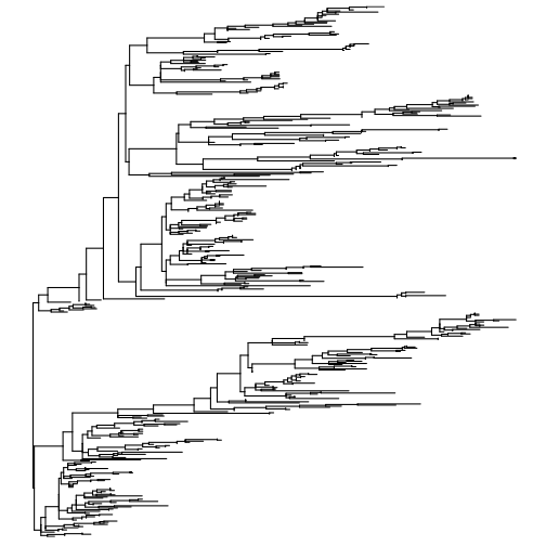
The resulting exported tree file is in Newick format (extension .nwk). Upload this tree file to the interactive tree of life tree viewer. This website offers very user friendly and sophisticated visualisation and manipulation of trees.
Viewing the tree should give you a feel for the diversity of bacterial taxa that exist in the sample but because the nodes in the tree are not assigned any taxonomic labels there is not much else we can say from looking at this tree. If we had a particular interest in one group of bacteria we might want to create a tree focussed on just that group and perhaps annotate the tree with colours or different sized points to indicate abundance. We won’t be doing that here, but keep in mind that this is one avenue of discovery that microbial researchers might explore in greater depth.
Optional (ggtree)
Also note that while ITOL is great there might come a point where you will want a package that can reproducibly produce publication quality trees directly from R and RMarkdown. The ggtree package is a great solution for making such high quality figures but it often requires quite a bit of work to adjust settings to get a nice result. Basic commands to visualise this tree using ggtree are shown below but ggtree is capable of much much more. Unfortunately we don’t have time to study ggtree in depth in this subject but if you are curious you may wish to consult the ggtree book
To install ggtree run the following code by pasting it into your R console (do not run this in an RMarkdown chunk because you will need to respond to prompts)
if (!requireNamespace("BiocManager", quietly = TRUE))
    install.packages("BiocManager")

BiocManager::install("ggtree")
To plot the tree
library(ggtree)

nwktree <- read.tree("qiime/rooted-tree/tree.nwk")

ggtree(nwktree)
Step 5 : Perform diversity analyses
Choose sampling depth
One of the critical aspects of diversity analyses is ensuring even sampling effort across samples. In practical terms this means that we need to pick a minimum cut-off for the number of sequences per sample. If a sample has more sequences than the cut-off a random subsample will be used. If a sample has fewer sequences than the cut-off it will be excluded from the analysis. If you are confused about this concept refer to your lecture notes. We cover it in this lecture.
Picking this number too low will result in loss of some low abundance sequences whereas picking it too high will result in loss of samples.
Use the qiime viewer to visualize qiime/table-deblur.qzv and use the interactive sample detail view to choose an appropriate value for minimum sampling depth. Don’t get too hung up on the exact value you choose here but as a general rule of thumb you should avoid removing more than a handful of samples.
Calculate diversity metrics
Run the code below to calculate diversity metrics. Important: Substitute the minimum sampling depth value you decided on above (the value of 200 shown below is not an ideal choice).
qiime diversity core-metrics-phylogenetic \
  --i-phylogeny qiime/rooted-tree.qza \
  --i-table qiime/table-deblur.qza \
  --p-sampling-depth 200 \
  --m-metadata-file raw_data/sample-metadata.tsv \
  --output-dir qiime/core-metrics-results
Look inside the qiime/core-metrics-results folder that this creates. It contains many files corresponding to different alpha and beta diversity metrics. Note that some .qzv files have already been created for you in here. You can download these and then visualise them with the qiime viewer https://view.qiime2.org/
Perform statistical analyses
Now use the alpha-group-significance plugin in qiime to perform a statistical test for association between Faith’s phylogenetic diversity and sample metadata. The test that will be performed is a Kruskal Wallis test which is the non-parametric equivalent of a one-way ANOVA. You can use this test to determine whether samples grouped according to a factor (eg body-site) come from the same distribution (the null hypothesis). A shorthand way of saying this is that it tests to see whether a grouping factor “is significant” in the sense that groups have different values of a response variable (eg alpha diversity). Run the code below and view the resulting visualisation.
Which experimental factors are significantly associated with Faith’s phylogenetic diversity?
qiime diversity alpha-group-significance \
  --i-alpha-diversity qiime/core-metrics-results/faith_pd_vector.qza \
  --m-metadata-file raw_data/sample-metadata.tsv \
  --o-visualization qiime/core-metrics-results/faith-pd-group-significance.qzv
Step 6 : Generate alpha rarefaction curves
When calculating diversity metrics we had to choose a value for the p-max-depth parameter. This parameter ensures even sampling depths (ie numbers of sequences) across samples. Here we explore what happens to alpha diversity metrics as a function of sampling depth. Intuitively, as depth increases so too should diversity, however this will only be true up to a point since eventually all of the actual biological diversity present in the sample will have been measured.
Run the code below to generate a visualisation for alpha rarefaction analysis
qiime diversity alpha-rarefaction \
  --i-table qiime/table-deblur.qza \
  --i-phylogeny qiime/rooted-tree.qza \
  --p-max-depth 4500 \
  --m-metadata-file raw_data/sample-metadata.tsv \
  --o-visualization qiime/alpha-rarefaction.qzv
Visualise the resulting alpha-rarefaction.qzv file using the qiime viewer. The default view separates the data from each barcode-sequence. These roughly correspond to the individual samples in the experiment. Set the metric to observed-features these correspond to ASVs in the analysis. Notice how this increases sharply at the left side of the plot (ie a small increase in sequencing depth will yield many more features). Also notice that there is quite a lot of difference between samples. Try switching the observed metric. Notice how some metrics continue to increase even at very high sequencing depth, whereas others (eg Shannon diversity) reach a plateau quite quickly.
Step 7 : Taxonomically classify sequences
One of the most useful aspects of sequencing based on the 16S gene is the fact that a very large number of other studies have also sequenced this gene. This includes many studies where the 16S gene has been sequenced for microbes of known taxonomy. By matching the sequences from our experiment against those of known taxonomy we can attempt to infer the taxonomy of our sequences.
In lectures we covered the theory behind taxonomic classification. (Relevant lecture here ). Here we will use a pre-built model ( fitted parameters for a Naive Bayesian classifier ) to perform classification.
First download the classifier and save it to the qiime directory
wget "https://data.qiime2.org/2023.5/common/gg-13-8-99-515-806-nb-classifier.qza" -O "qiime/gg-13-8-99-515-806-nb-classifier.qza"
Run the classifier using the feature-classifier classify-sklearn plugin in qiime.
Edit the code below to run this plugin. First run the code as-shown. This will show the options available and also produce errors that list missing options that are mandatory. Edit the code to run this plugin correctly by providing all of the mandatory options.
Note: For the --i-reads option you should use the rep sequences generated by deblur
qiime feature-classifier classify-sklearn --o-classification qiime/taxonomy.qza
Now create a barplot visualisation for your resulting taxonomy file using the code below.
qiime taxa barplot \
  --i-table qiime/table-deblur.qza \
  --i-taxonomy qiime/taxonomy.qza \
  --m-metadata-file raw_data/sample-metadata.tsv \
  --o-visualization qiime/taxa-bar-plots.qzv
Explore the barplot visualisation you in the qiime viewer https://view.qiime2.org/
What is the dominant taxonomic group (at Level 2; Phylum) in the human gut? How does this differ from other body sites?
Answers to questions
Code to incorporate sample metadata in the feature table summary visualisation
qiime feature-table summarize \
  --i-table qiime/table-deblur.qza \
  --m-sample-metadata-file raw_data/sample-metadata.tsv \
  --o-visualization qiime/table-deblur.qzv
Code to run a mafft alignment
qiime alignment mafft \
  --i-sequences qiime/rep-seqs-deblur.qza \
  --o-alignment qiime/aligned-rep-seqs.qza
Code to run the sklearn feature classifier
qiime feature-classifier classify-sklearn \
  --i-classifier qiime/gg-13-8-99-515-806-nb-classifier.qza \
  --i-reads qiime/rep-seqs-deblur.qza \
  --o-classification qiime/taxonomy.qza