BC3203
Goal
The goal of this tutorial is to introduce you to some key tools used in variant analysis. This includes both command-line and graphical tools. The focus will be on understanding how to extract biologically or clinically useful information from the data.
Prior Reading and Reference Material
This tutorial relies on general command-line skills as well as some understanding of the sam/bam format. The guide re-introduces these concepts but if you would like further information please revisit the RNASeq assignment (which analyses a bam file).
Completing the assessment
Unlike previous tutorials there are no automated tests. Instead you will be required to write your answers in markdown format directly into the exercises.Rmd file. Prior to uploading your answer please knit this file. It should produce a file called exercises.md which you should add to git and include in your submission to github. I will be able to read this and mark it directly by visiting your github page.
Note that there is no need to provide long answers for these exercises. Some answers require just a single line of text, others may require a small block of code or perhaps a few lines of text. Be sure to read the question carefully and answer it as directly as possible.
Guide
This guide walks through two examples of variant analysis with a focus on those that arise due to denovo mutations. Since variant analysis and RNA seq both make use of read alignment data some of the tools (eg samtools) and data formats (sam/bam) encountered in the RNA seq assignment will be encountered again.
How to complete this guide
Complete this guide by following all the steps from top to bottom.
All of the commands that you need to run are written in code blocks. Since some commands are quite long and complex to type you have been provided with a copy of all commands in the file commands.Rmd. Feel free to use this file as an easy way to run commands. You may also wish to make notes in this file for your own use. This file does not need to be submitted as it is just for your convenience.
Great care has been taken to ensure that the commands in this guide will run fairly quickly. This will allow you to get a feeling for the steps involved but is only possible because we are using extremely cut-down input data. For a real analysis the computational resources required would be many orders of magnitude higher.
Before you start!
Make sure you run the setup script. This will download the example data
bash setup.sh
Part 1: Cancer Variants
This section focusses on paired tumour/normal analysis. This is an important tool in understanding cancer itself as well as in clinical settings where analysis of variants can indicate prognosis and/or preferred treatments.
In the tumour/normal context the focus is usually on somatic mutations. These are mutations that are not inherited because they occur in normal body cells. They are often associated with cancer and indeed part of the mechanism by which tumours arise is as a result of an accumulation of somatic mutations leading to a line of cells that has the hallmarks of cancer.
Most cancers carry many thousands of somatic mutations. A good way to detect these is by comparing the genome of tumour cells with normal cells from the same patient and that is what we will do in this analysis.
First create a subdirectory to keep all of the files related to this section of the analysis “Cancer Variants”.
mkdir -p cache/cancer
Important Note
All of the commands in this section of the guide will be run from within cache/cancer. In some cases you will see commands like cd cache/cancer at the top of the example code block in this guide. In those cases you can just run the code by clicking run directly in RMarkdown. If you don’t see cd cache/cancer it means you need to be inside the cache/cancer directory and should run the command by cut-pasting from the guide into the Terminal.
Setup the Analysis Directory
Now setup access to all required files within the cache/cancer directory. This is done by creating symbolic links from the originals to that directory. Copy and paste the entire code block below to do this.
The ln command is used here to create symbolic links. A symbolic link is a tiny file that simply instructs the filesystem to look elsewhere for the original version of the file. Instead of making copies of large files it is often much better to use a symbolic link. This also allows you to organise your analyses without moving original data.
Note that if you run this twice it will refuse to overwrite any links that already exist and give an error like ln: <file>: File exists. Don’t worry about these errors.
cd cache/cancer

# This is a database of known Human snps. Used for base call score recalibration
#
ln -s ../../data/dbsnp_138.b37.small.vcf .

# The human genome reference and associated index files
#
ln -s /pvol/data/variants/GRCh37.fa .
ln -s /pvol/data/variants/GRCh37.fa.fai .
ln -s /pvol/data/variants/GRCh37.dict .

# A file with start and end positions for human chromosome 11
#
ln -s ../../data/11.intervals .

# Indexed bam files with reads from tumour and normal samples aligned to the human genome
#
ln -s ../../data/normal.bam .
ln -s ../../data/tumour.bam .
ln -s ../../data/normal.bam.bai .
ln -s ../../data/tumour.bam.bai .
Exploring BAM files
The reads for this analysis are contained within two files labelled normal and tumour respectively. They are in BAM format. BAM is just a binary compressed version of SAM which is effectively a tab separated table (potentially very large) where each row represents an alignment of a read to a reference sequence. Detailed information on the format is provided on this wikipedia entry and the official sam format specification
Try looking at the first 5 lines of the file normal.bam. This can be done using the samtools view command;
samtools view normal.bam | head -n5
Unfortunately each line is quite long so it is difficult to see that this is just a tabular file. Nevertheless, if you look carefully you will be able to see that there are around 20 columns. The first 11 columns are mandatory so they are found in every sam/bam file. The remaining columns are optional and allow extra information to be encoded about each alignment.
| Col | Field | Type | Brief Description |
|---|---|---|---|
| 1 | QNAME | String | Query template NAME (Name of the read) |
| 2 | FLAG | Int | bitwise FLAG |
| 3 | RNAME | String | References sequence NAME |
| 4 | POS | Int | 1- based leftmost mapping POSition |
| 5 | MAPQ | Int | MAPping Quality |
| 6 | CIGAR | String | CIGAR String |
| 7 | RNEXT | String | Ref. name of the mate/next read |
| 8 | PNEXT | Int | Position of the mate/next read |
| 9 | TLEN | Int | observed Template LENgth |
| 10 | SEQ | String | segment SEQuence |
| 11 | QUAL | String | ASCII of Phred-scaled base QUALity+33 |
Now lets explore the second column which contains an integer valued field called the FLAG. The values in this column cleverly encode a great deal of information in a single number. For example a value of 4 means that the read is unmapped, a value of 68 means it is unmapped and also the first in a pair of reads. The easiest way to translate between these flags and their meanings is to use an online tool available at https://broadinstitute.github.io/picard/explain-flags.html . Be sure to open a webpage with that tool for the next section.
Use the following command to cut only the second column (containing the flag) from the file
samtools view normal.bam | head -n5 | cut -f2
Notice that several of the values are repeated. It might be interesting to see a list of all the flag values in the file. To obtain this we can use the sort and uniq tools.
The command below will produce a table of all FLAG values in the file along with a count of how many times they occurred. The first column is the count, the second is the FLAG value.
samtools view normal.bam | cut -f2 | sort -n | uniq -c | sort -n -r
Explore some of these values using the explainflags web tool.
Question 1
The four most common FLAG values represent the majority of alignments in the file. What two things do all of the reads with these four flags have in common.
Now examine the alignment for a specific read pair, D9S4KXP1:329:C72TCACXX:4:2110:4463:45409. This can be done using grep to search for the read name in the sam output.
samtools view normal.bam | grep 'D9S4KXP1:329:C72TCACXX:4:2110:4463:45409'
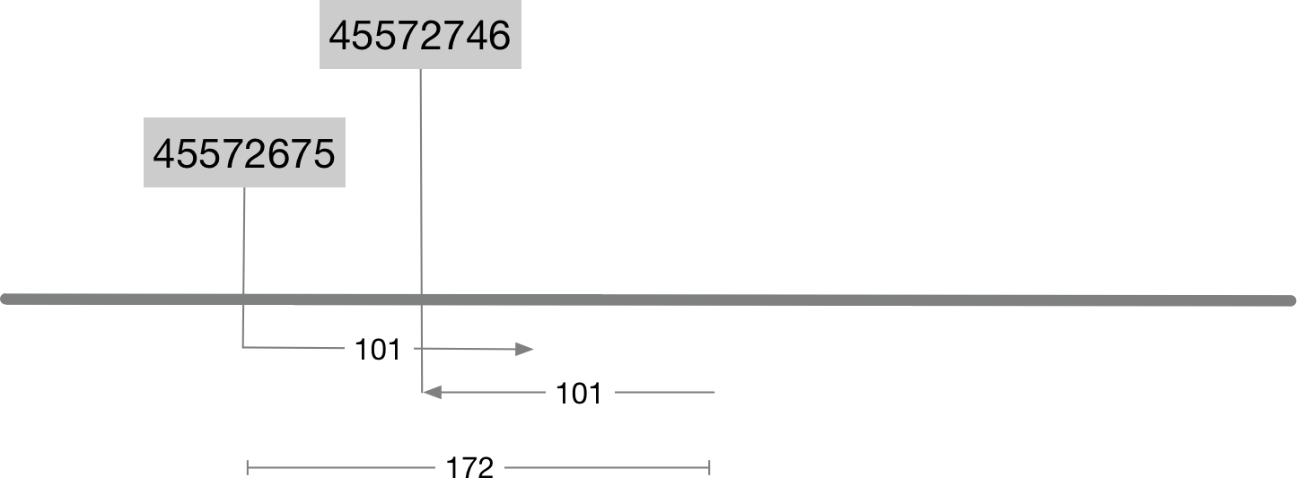
Note that this prints out a pair of alignments because this name belongs to a paired read. Information about the position and alignment of these reads is shown graphically in the image below. Look carefully at the image and make sure you can reconcile the information in columns 4, 6 and 9 with the image.
- The value in column 4 is the alignment start position.
- The value in column 6 is the CIGAR string.
101Mmeans there are 101 bases and all are alignment matches. - The value in column 9 is the
template length. Also referred to as theinsert size. It is closely related to the size of the original DNA fragments that were sequenced. In paired end sequencing the reads will start at either end of this fragment and be sequenced inwards.
Question 2
Although the template length or insert size is reported directly in column 9 it can also be calculated purely using the alignment coordinates and the cigar string? How would you do this? Write your answer as a simple R command (eg 34-65+100)
Indel Realignment
The next step in preparing the BAM file for variant calling is to realign around indels and snp dense regions. The idea behind this step is that regions with indels and high snp density tend to result in more alignment errors. Normally alignment is performed one read at a time but for problematic regions a better strategy is to calculate an optimal alignment (minimising mismatches) across all of the reads together. This is obviously not practical to perform (for computational reasons) across an entire genome but can be done for specific regions.
The Genome Analysis toolkit (GATK) has a tool for this called IndelRealigner which runs in 2 steps.
The first step finds target regions where realignment should be performed (ie regions around indels and where SNP density is high). Run the code below to perform this step. It will result in a file called realign.intervals containing the intervals to be realigned.
gatk -T RealignerTargetCreator\
  -R GRCh37.fa -I normal.bam -I tumour.bam -L 11.intervals -o realign.intervals
Question 3
How many regions were identified by RealignerTargetCreator as needing realignment?
The second step actually performs the realignment and results in the production of new bam files, one for the tumour sample and another for normal.
gatk -T IndelRealigner -R GRCh37.fa -I normal.bam -I tumour.bam -L 11.intervals -targetIntervals realign.intervals --nWayOut .realigned.bam
Question 4
How many alignments are there in normal.bam? How many in normal.realigned.bam?
Hint: Use samtools view to print the alignments in a .bam file with one alignment per line.
Almost all of the commands in this tutorial come from two large software packages that often work together, GATK and Picard, both developed at the broad institute. The are software suites consisting of many tools that work together and share a common set of options. Here is an explanation of core options in the programs run so far;
| Option | Meaning |
|---|---|
| -T | GATK algorithm to run |
| -R | the reference genome used for mapping (GRCh37) |
| -L | Genomic intervals to operate on |
Mark Duplicates
One of the fundamental assumptions of variant calling algorithms is that all of the reads are independent samples from across the genome. One way that this assumption can be violated is if the same fragment of DNA is sequenced twice. This usually occurs due to low library complexity (ie too few different fragments of DNA after PCR amplification) but it can also occur if a single cluster on the instrument is interpreted as two separate clusters (optical duplicate).
The MarkDuplicates tool detects both PCR and Optical duplicates by examining the 5’ ends of the reads as well as their quality scores. See documentation for MarkDuplicates for more info.
Mark duplicates for the tumour and normal samples by running the commands below.
picard MarkDuplicates ASSUME_SORTED=TRUE REMOVE_DUPLICATES=false CREATE_MD5_FILE=true VALIDATION_STRINGENCY=SILENT CREATE_INDEX=true INPUT=normal.realigned.bam OUTPUT=normal.markdup.bam METRICS_FILE=normal.dup.metrics

picard MarkDuplicates ASSUME_SORTED=TRUE REMOVE_DUPLICATES=false CREATE_MD5_FILE=true VALIDATION_STRINGENCY=SILENT CREATE_INDEX=true INPUT=tumour.realigned.bam OUTPUT=tumour.markdup.bam METRICS_FILE=tumour.dup.metrics
Question 5
What percent of reads are duplicated in the tumour sample? Hint: Look at the metrics file created (eg tumour.dup.metrics)
Base Recalibration
Sequencing vendors tend to inflate the quality of bases generated. We run base recalibration to lower the score for certain motifs known to have biases for different technologies.
We need to do this both for the tumour and the normal again. Instead of running two separate commands we can use a for loop that repeats the same operation for a list of items.
for f in tumour normal; do
	gatk -T BaseRecalibrator -nct 2 -R GRCh37.fa -L 11.intervals -knownSites dbsnp_138.b37.small.vcf -I ${f}.markdup.bam -o ${f}.recal;
	gatk -T PrintReads -nct 2 -R GRCh37.fa -BQSR ${f}.recal -I ${f}.markdup.bam -o ${f}.recal.bam ;
done
BAM QC
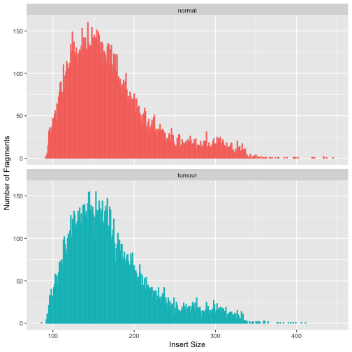
Once your whole bam is generated, it’s always a good thing to check the data again to see if everything makes sense. Let’s first examine the insert size. It corresponds to the size of DNA fragments sequenced. Note that this is different from the gap size (= distance between reads) !
The command below will use a Picard tool CollectInsertSizeMetrics to gather statistics on insert sizes
for f in tumour normal; do
	picard CollectInsertSizeMetrics \
	I=${f}.recal.bam O=${f}.insertSize H=${f}_insertSize.pdf \
	METRIC_ACCUMULATION_LEVEL=LIBRARY M=0.5;
done
The following code can be used to read the insert size metrics and plot the histogram computed by the tool.
library(tidyverse)
is_normal <- read_tsv("cache/cancer/normal.insertSize",skip = 11) %>% add_column(sample="normal") %>%
  rename(lib_fr_count=`normal_lib.fr_count`)
is_tumour <- read_tsv("cache/cancer/tumour.insertSize",skip = 11) %>% add_column(sample="tumour") %>%
  rename(lib_fr_count=`tumour_lib.fr_count`)
insert_size_data <- rbind(is_normal,is_tumour)

ggplot(insert_size_data,aes(x=insert_size)) +
  geom_col(aes(y=`lib_fr_count`, color=sample)) +
  facet_wrap(~sample,ncol = 1) +
  xlab("Insert Size") + ylab("Number of Fragments") +
  guides(color="none")
Variant Calling
Variant calling involves statistical evaluation of the reads aligned at a particular position in the genome to determine whether a variant exists at that position. Single nucleotide variants (SNV) are probably the simplest to call, but even for this category there are many approaches including Bayesian, a threshold or a t-test approach.
Here we will try 2 variant callers.
- Varscan2
- MuTecT2
First let’s try MuTect2 which is part of the GATK suite. This command takes a few minutes to run.
gatk -T MuTect2 -R GRCh37.fa -L 11.intervals -I:tumor tumour.recal.bam -I:normal normal.recal.bam -o mutect2.vcf
Note that the output is a file, mutect2.vcf in VCF format. VCF is the standard format for storing sequence variation information. Like many of the bioinformatic formats we have encountered it is essentially tabular (with some non-tabular header rows). Each row in VCF represents a variant with tab delimited columns as follows:
| Field | Name | Brief description (see the specification for details) |
|---|---|---|
| 1 | CHROM | The name of the sequence on which the variation is being called. |
| 2 | POS | The 1 based position of the variation on the given sequence. |
| 3 | ID | The identifier of the variation, or if unknown a . |
| 4 | REF | The reference base at the given position on the reference sequence. |
| 5 | ALT | The list of alternative alleles at this position. |
| 6 | QUAL | A quality score associated with the inference of the given alleles. |
| 7 | FILTER | A flag indicating which of a given set of filters the variation has passed. |
| 8 | INFO | An extensible list of key-value pairs describing the variation. |
| 9 | FORMAT | An extensible list of fields for describing the samples. |
+ |
SAMPLEs | For each sample described in the file, values are given for the fields listed in FORMAT |
Now let’s run varScan2. VarScan calls somatic variants (SNPs and indels) using a heuristic method and
a statistical test based on the number of aligned reads supporting each allele. The Varscan somatic caller expects both a normal and a tumour file in SAMtools pileup format from sequence alignments in binary alignment/map (BAM) format.
Use the following command to build a separate pileup file for tumour and normal.
for f in tumour normal; do
	samtools mpileup -L 1000 -q 1 -f GRCh37.fa -r 11 ${f}.recal.bam > ${f}.mpileup;
done
Once the pileup files are generated we can call variants with VarScan using the command below;
varscan somatic normal.mpileup tumour.mpileup varscan2 --output-vcf 1 --strand-filter 1 --somatic-p-value 0.001
Varscan generates a series of output files with the prefix varscan. This includes two separate vcf’s. One for indels and another for SNPs.
Inspecting Variants
Now explore the variants found by varscan2 and mutect. We are specifically interested in somatic variants. In the varscan output these are annotated with the SOMATIC flag so we can simply use grep to find them like this
grep SOMATIC varscan2.snp.vcf | grep -v ^#
Mutect2 is specifically designed to detect somatic variants so we just need to filter for variants that PASS its filtering criteria. Again this can be done with grep like so;
grep PASS mutect2.vcf
Question 6
Look at the positions of the variants identified by Mutect2 and VarScan. How many variants are there in common?
Variant Visualisation
The Integrative Genomics Viewer (IGV) is an efficient visualization tool for interactive exploration of large genome datasets.
To run IGV do the following;
- Go to IGV web application on https://igv.org/app/ .
- Select the correct reference genome (human GRCh37/hg19)
- Prepare indexes for the tumour and normal BAM files
  samtools index tumour.realigned.bam
  samtools index normal.realigned.bam
- Download tumour and normal BAM files from rstudio onto your computer (see here for how).
- In step 4 make sure you download the indexes as well (ie tumour.realigned.bam, tumour.realigned.bam.bai). Keep them all in the same folder on your computer.
- Load the tumour and normal BAM files. Select both bam files and their indexes together for a single upload.
To investigate differences between algorithms let’s visually interrogate some of these variants. First, let’s look at a variant called by both algorithms.
Enter chr11:45671776 into the region text box. To view a summary of all the reads aligned at a particular base click (or hover your mouse on) the coverage track.
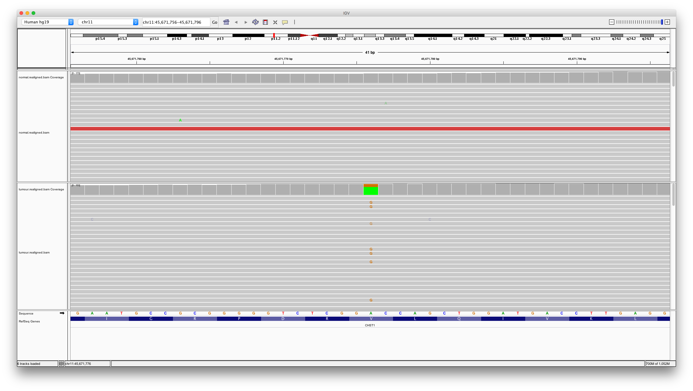
Question 7
Does this look like a real somatic mutation? How many variant bases are detected in the normal? How many in the tumour?
Question 8
Typically heterozygous mutations should be present in about half of the aligned reads? Consider the proportion of variant reads in the tumour sample (40/140). What might explain this number?
Now let’s look at a variant only detected by mutect. Enter chr11:129061849 into the region box.
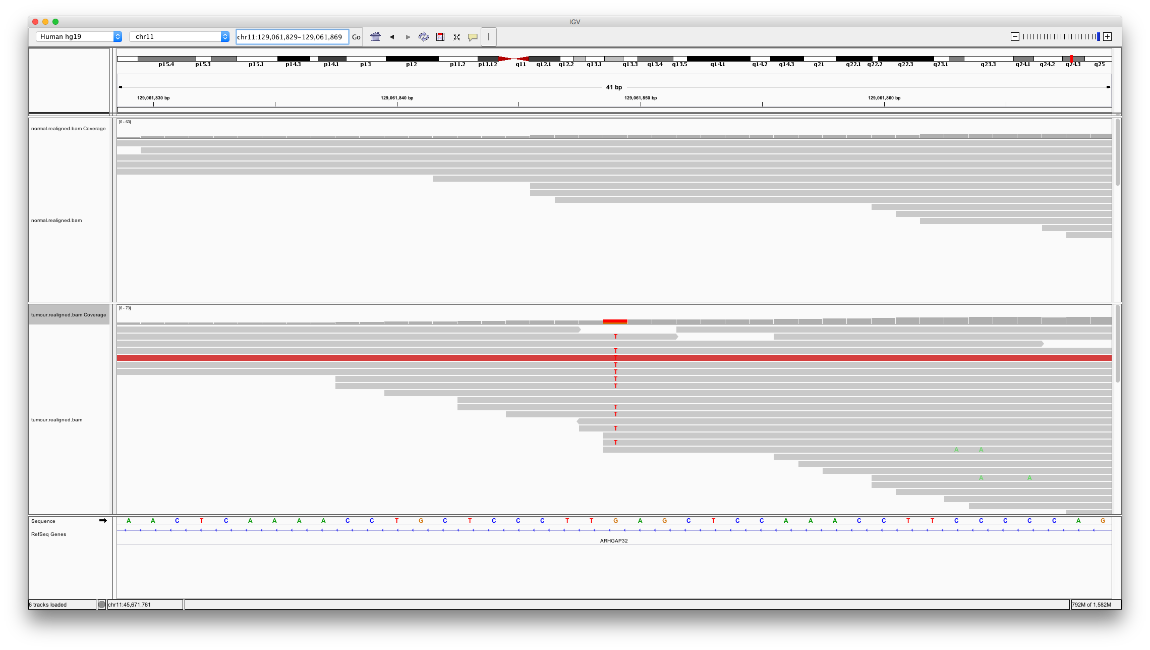
Question 9
Does this variant look real and somatic? Why might varscan2 not have called it?
Hint: consider the read depth in the region of this variant compared to what was seen for the previous example
Now let’s consider a somatic variant call unique to varscan2. Enter chr11:67742248
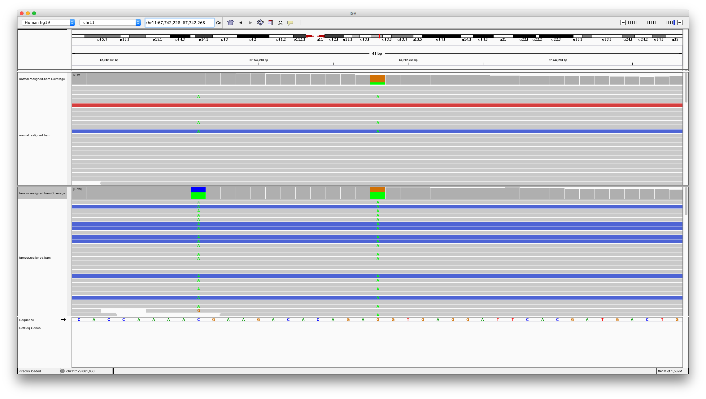
Question 10
Does this variant look somatic? Are there are other potential issues with this region of the genome?
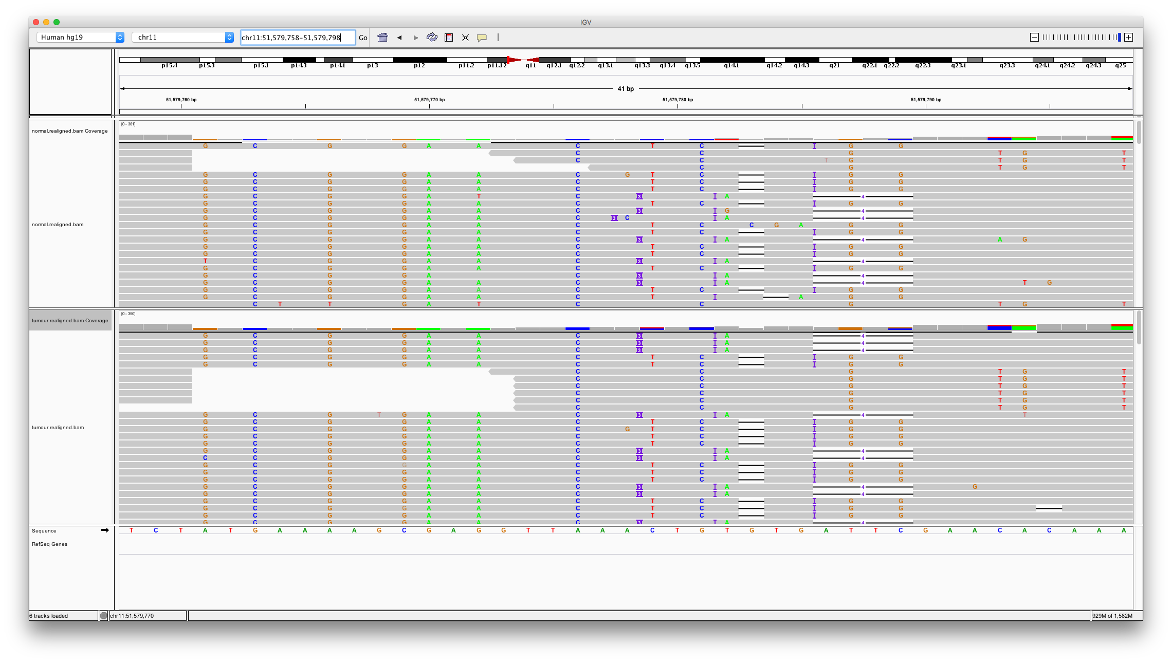
Now let’s examine a problematic region for alignment. Varscan2 calls a 3bp insertion at chr11:51579778. Enter these coordinates. We can quickly there are numerous issues with aligning to this region. Many variant callers won’t call variants in regions like this but unfortunately varscan has.
Part 2: Germline Variant Analysis
This section focusses on germline mutations. In contrast to somatic mutations these arise during the production of gametes (sperm or egg) or very early in the development of an individual. They are therefore carried by all cells within an individual.
In this analysis we will detect germline mutations in a child by combining data from the child with that of both its parents. Since germline mutations arise during gamete production they are not carried by the parents but will be carried by the child.
First make sure you are in the top level of your project directory. If you are in cache/cancer you can do this as follows
cd ../../
Next create a new subdirectory to keep files related to this section of the analysis “Germline Variants”.
mkdir -p cache/germline
cd cache/germline

# Samples from mother, father and child
#
ln -s ../../data/child.bam .
ln -s ../../data/mother.bam .
ln -s ../../data/father.bam .
ln -s ../../data/child.bam.bai .
ln -s ../../data/mother.bam.bai .
ln -s ../../data/father.bam.bai .

# The human genome reference and associated index files
#
ln -s /pvol/data/variants/GRCh37.fa .
ln -s /pvol/data/variants/GRCh37.fa.fai .
ln -s /pvol/data/variants/GRCh37.dict .
The following command uses samtools to generate a pileup file based on alignments in bam files from mother.bam, child.bam and father.bam.
samtools mpileup -B -q 1 -L 1000 -f GRCh37.fa -r 17:7000000-8000000 father.bam mother.bam child.bam > trio.mpileup
The trio analysis can then be performed with VarScan
varscan trio trio.mpileup trio.mpileup.out --min-coverage 10 -- min-var-freq 0.20 --p-value 0.05 -adj-var-freq 0.05 -adj-p-value 0.15
The candidate denovo (germline) mutations can be found using grep
grep 'DENOVO' trio.mpileup.out.snp.vcf
Note that in addition to the two detected variants this also shows a header line explaining the meaning of the DENOVO flag.
This shows two locations in the genome that might be denovo mutations;
chr17:7459297chr17:7574017
Open IGV and load bam files for child, father and mother. Inspect these two locations
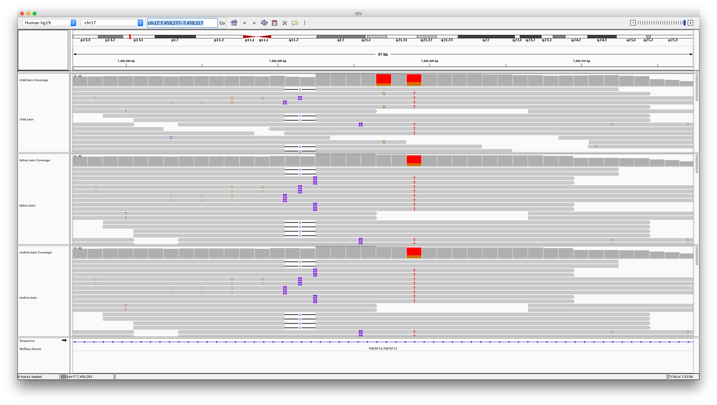
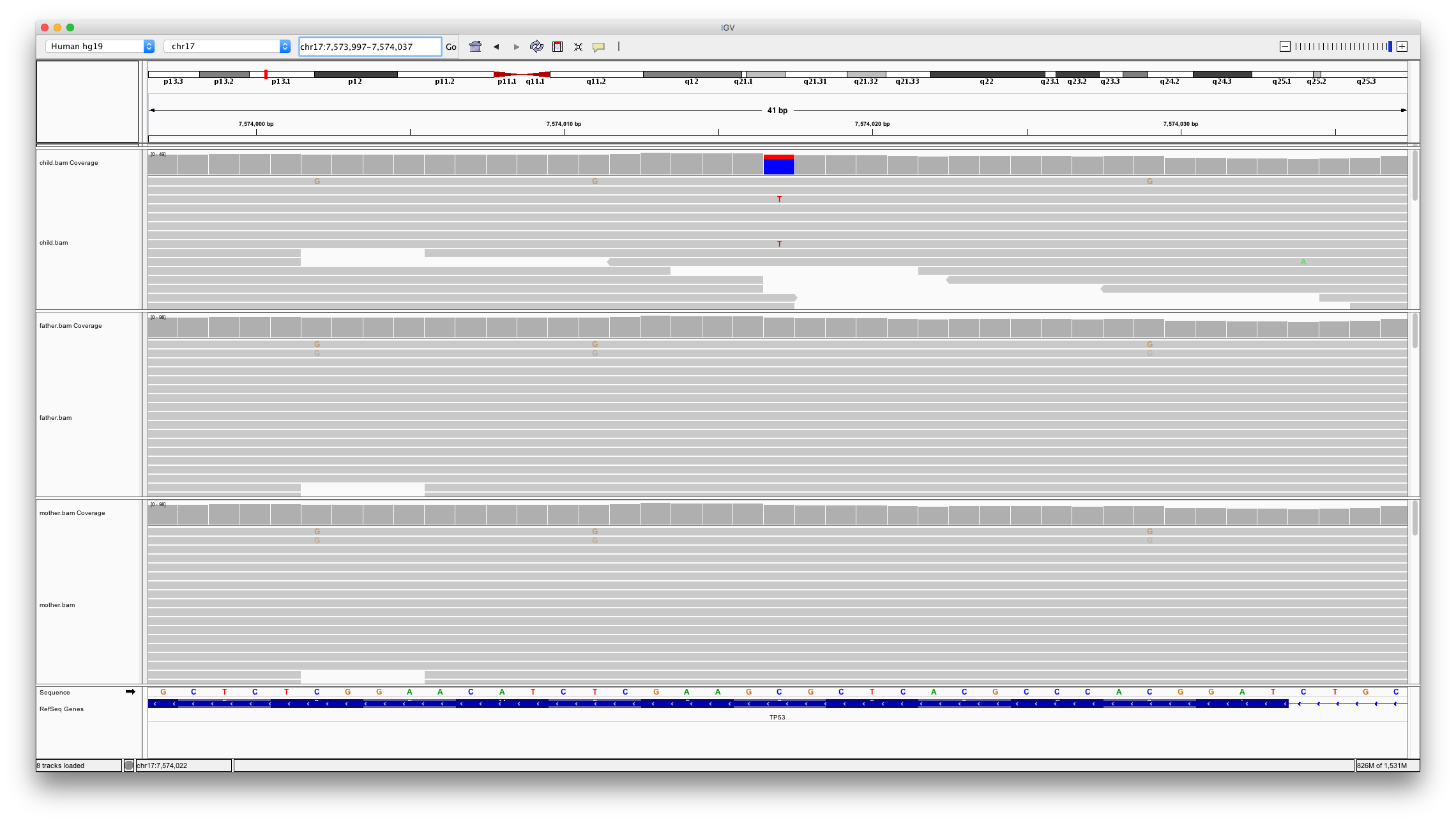
Question 11
Which of the variants looks to be a real denovo mutation and why?
Variant Annotation
There looks to be one real denovo mutation so let’s annotate this variant to see if it’s likely to be causal.
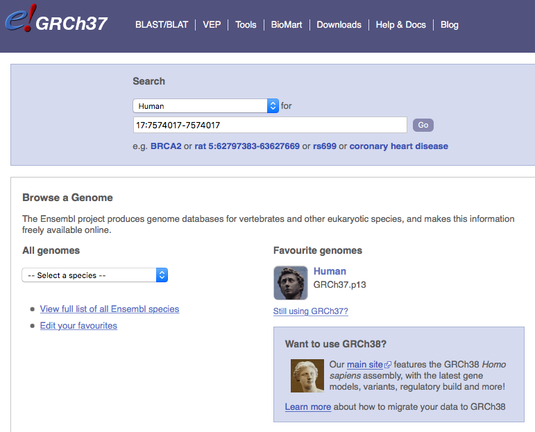
Let’s first use ensembl to examine this region. Go to http://grch37.ensembl.org/index.html, select human and enter 17:7574017-7574017 into the search box.
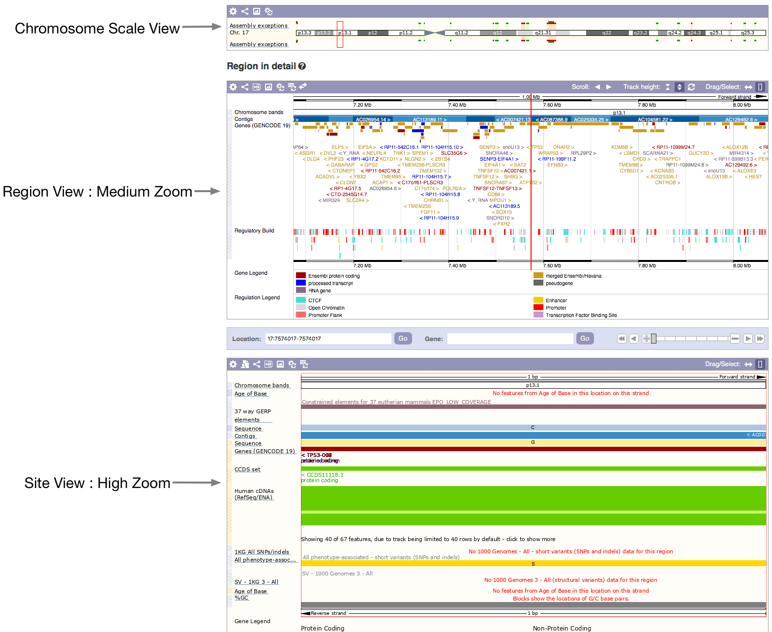
Browse and scroll around to get a feel for the information included in each of the three panes. The first is a chromosome—scale view, showing the chromosome arms and banding pattern, below this is an enlargement of the region shown in the red box on the chromosome view. This shows the gene landscape in the chromosomal region. The third pane shows the region you specified with coordinates for your search. The bars represent gene transcripts in this small region. Reading the labels, we can see that this gene has the gene symbol TP53.
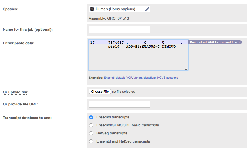
Since our variant occurs within the gene TP53 we would like to know what effect it might have on the function of that gene. One tool for this is variant effect predictor (VEP). Go to the VEP web page at http://grch37.ensembl.org/Homo_sapiens/Tools/VEP?db=core
As input VEP allows us to enter a line from a VCF file. Enter the vcf entry corresponding to our causal variant (identified with grep above) into VEP. Leave all other parameters as is and click run near the bottom of the page. When the analysis lists as done, click on ‘View results’. There are lots of different transcripts for TP53 and we see a consequence for each of these with the most damaging listed first.
Question 12
Looking at the results for the top entry only. What is the consequence of this SNV? What exon is the variant found in? Is the variant previously reported? What is the amino acid position of the protein and what is the amino acid change?
Note: You will need to scroll to the right to answer this question as the table is very wide
Clinical Interpretation
You’ve received a clinical report stating that the child exhibits symptoms of Li-Fraumeni Syndrome. Now we have a candidate variant let’s explore our disease in more detail to make sure the information agrees.
Let’s learn a bit about this disease and examine if our variant may be causing this. The databases are important resources that are our best collections and compilations of research and clinical data about mutations and human disease.
First let’s examine Orphanet https://www.orpha.net/consor/cgi-bin/index.php Enter Li-Fraumeni Syndrome in the search box and then click the link to the Orphanet database describing Li-Fraumeni Syndrome. Read the first few paragraphs of the main entry.
From the Orphanet page for Li-Fraumeni Syndrome, click the first link to the OMIM database (click here if you can’t find these). Briefly read through this page and learn of the striking clinical features of this disease that led to its identification. Click on the ‘Inheritance’ link of the disease.
Find the ‘external links’ section in the right hand margin of the OMIM Li-Fraumeni Syndrome top page. Click on the ‘Protein’ and ‘UniProt’ links.
Once in UniProt, choose the protein entry ‘P53_HUMAN’ (if you get stuck, go here ).
Listed in a very long page is a gold-mine of information. Not all UniProt entries are as long, but TP53 is a very well studied protein.
Find the ‘Pathology and Biotech’ section on this page. This contains a description of diseases that mutations/variations in TP53 cause. It also helpfully lists all observed variation and links these to the publications that first described them. Scrolling down in this section further you will find a table of induced mutations in this gene and their functional consequence.
Question 13
Can you find our mutation in the table? How many mutations are reported at the amino acid? Are there any publications reported for our mutation?
Hint: remember the amino acid position from earlier.
Congratulations you’ve discovered the causal variant in this pedigree. The next step is to report this information to the clinician treating the child and they will investigate whether this variant is ‘actionable’. Actionable means there are guidelines regarding treatment in patients with the variant.